PivotTable's Report Filter using "greater than"
Categories:
Applying 'Greater Than' Filters in Excel PivotTable Report Filters

Learn how to effectively use 'greater than' criteria within Excel PivotTable report filters to analyze data dynamically and extract meaningful insights.
Excel PivotTables are powerful tools for summarizing and analyzing large datasets. While basic filtering options are straightforward, applying advanced criteria like 'greater than' directly within the Report Filter (now often called 'Filter' or 'Slicer' depending on Excel version and context) can sometimes be less intuitive. This article will guide you through the process of setting up a 'greater than' filter for numerical data in your PivotTable's report filter area, enabling more dynamic and precise data analysis.
Understanding PivotTable Filters
PivotTables offer several filtering mechanisms:
- Report Filters (or Slicers): These apply filters to the entire PivotTable, allowing you to view data for specific categories or conditions. They are typically placed at the top of the PivotTable.
- Row/Column Label Filters: These filter the visible rows or columns based on their labels.
- Value Filters: These filter rows or columns based on the aggregated values in the data area.
Our focus here is on applying a 'greater than' condition to a field placed in the Report Filter area. This is particularly useful when you want to quickly switch between different thresholds for your entire report.
flowchart TD
    A[Start with Raw Data] --> B{Create PivotTable}
    B --> C[Drag Field to 'Filters' Area]
    C --> D{"Click Filter Dropdown (in PivotTable)"}
    D --> E{"Select 'Number Filters'"}
    E --> F["Choose 'Greater Than...'" ]
    F --> G["Enter Value and Confirm"]
    G --> H[PivotTable Filters Data]
    H --> I[End]
Workflow for applying a 'Greater Than' filter in a PivotTable Report Filter.
Step-by-Step: Applying a 'Greater Than' Report Filter
Let's walk through the process of setting up a 'greater than' filter. Assume you have a dataset with a 'Sales Amount' column and you want to filter your entire PivotTable to show only data where the sales amount exceeds a certain value.
1. Prepare Your PivotTable
Ensure you have an existing PivotTable. If not, select your data range, go to 'Insert' > 'PivotTable', and place it on a new or existing worksheet. Drag the numerical field you wish to filter (e.g., 'Sales Amount') into the 'Filters' area of the PivotTable Fields pane.
2. Access the Filter Options
On your PivotTable, locate the dropdown arrow next to the field you placed in the 'Filters' area (e.g., 'Sales Amount'). Click this dropdown arrow to reveal the filtering options.
3. Select 'Number Filters'
In the dropdown menu, hover over 'Number Filters'. This will open a sub-menu with various numerical comparison options.
4. Choose 'Greater Than...'
From the 'Number Filters' sub-menu, select 'Greater Than...'. A 'Custom AutoFilter' dialog box will appear.
5. Enter the Threshold Value
In the 'Custom AutoFilter' dialog box, ensure the first dropdown is set to 'is greater than'. In the adjacent input box, type the numerical value you want to use as your threshold (e.g., 5000). Click 'OK'.
6. Observe the Filtered Data
Your PivotTable will now update to display only the data that meets the 'greater than' criterion you specified. The filter icon next to your field in the 'Filters' area will change to indicate that a custom filter is active.
Common Pitfalls and Troubleshooting
Sometimes, the 'Number Filters' option might be greyed out or not behave as expected. Here are a few things to check:
- Data Type: Ensure the field you are trying to filter is recognized as a numerical data type in your source data. If it contains text or mixed data, Excel might treat it as text, disabling number filters.
- Refresh PivotTable: After making changes to your source data, always refresh your PivotTable ('Analyze' tab > 'Refresh') to ensure the filter options are up-to-date.
- Field Placement: The 'Number Filters' option is typically available for fields placed in the 'Rows', 'Columns', or 'Filters' areas. If your field is in the 'Values' area, you'll use 'Value Filters' instead, which also offers 'greater than' options but applies to the aggregated results.
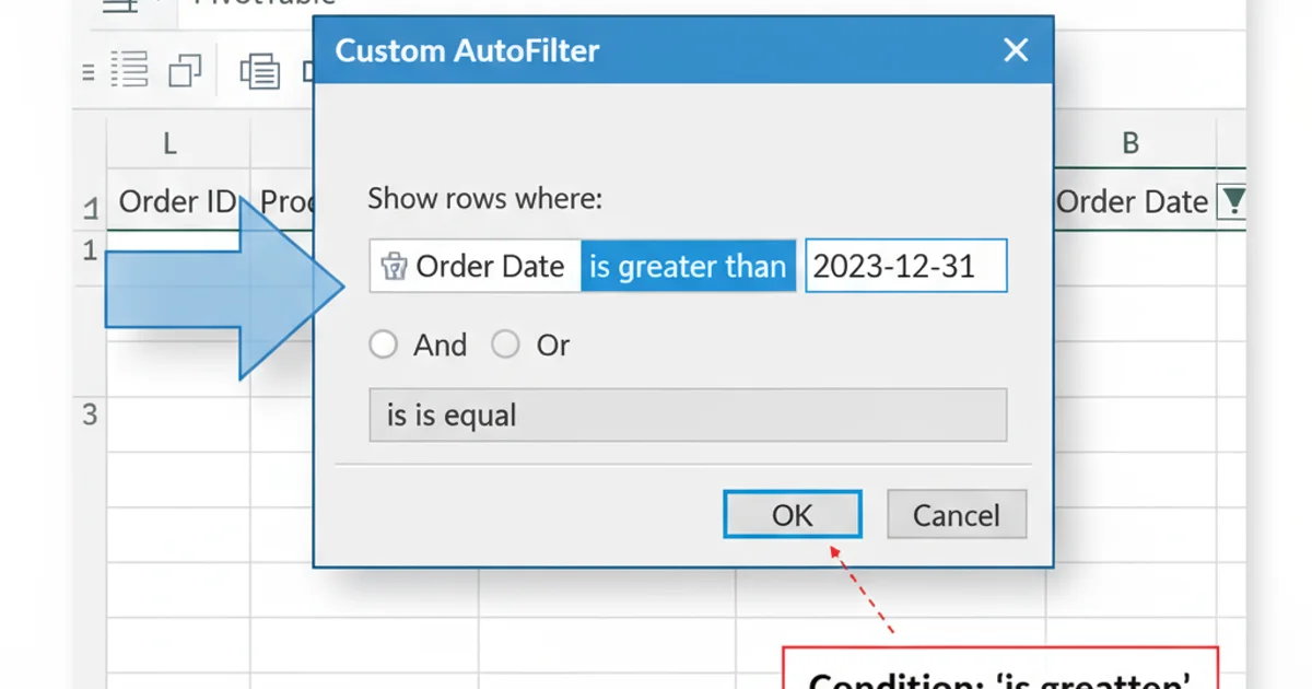
The 'Custom AutoFilter' dialog box allows you to define specific numerical conditions.
Mastering advanced filtering in PivotTables, especially with conditions like 'greater than', significantly enhances your ability to perform targeted data analysis. By following these steps, you can efficiently segment your data and gain deeper insights from your reports.