Use Excel pivot table as data source for another Pivot Table

Using an Excel Pivot Table as a Data Source for Another Pivot Table

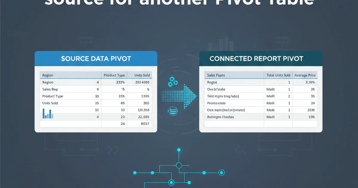
Learn how to leverage an existing Excel Pivot Table's results as the data source for a new, secondary Pivot Table, enabling multi-stage analysis and complex reporting.

Excel Pivot Tables are powerful tools for summarizing and analyzing large datasets. However, sometimes the insights you need require a multi-stage analysis, where the output of one Pivot Table serves as the input for another. While Excel doesn't directly allow you to select a Pivot Table's output range as the source for a new Pivot Table, there are effective workarounds to achieve this, primarily by converting the first Pivot Table's output into a static range.

Why Use a Pivot Table as a Source?

The primary reason to use a Pivot Table's output as a source for another is to perform further aggregation or analysis on already summarized data. This is particularly useful when:

• Complex Calculations: You need to apply additional calculations or groupings that are difficult to implement directly in the first Pivot Table.
• Data Cleansing/Transformation: The first Pivot Table performs a necessary aggregation or transformation (e.g., grouping dates, categorizing items) that then needs to be analyzed further.
• Reporting Structure: You want to present data in a specific hierarchical or summarized way that requires multiple layers of pivoting.
• Performance: For very large datasets, pre-summarizing data with a Pivot Table can make subsequent analysis faster.

flowchart TD
    A["Raw Data (e.g., Sales Transactions)"] --> B["First Pivot Table (e.g., Sales by Region)"]
    B --> C{"Copy & Paste as Values"}
    C --> D["Static Data Range (Output of First PT)"]
    D --> E["Second Pivot Table (e.g., Regional Performance Analysis)"]
    E --> F["Final Report/Analysis"]

Workflow for using a Pivot Table's output as a source for another

Method 1: Copy and Paste as Values

This is the most straightforward and commonly used method. It involves taking the summarized data from your first Pivot Table and pasting it as static values into a new range. This new static range then becomes the data source for your second Pivot Table.

1. Create Your First Pivot Table

Start by creating your initial Pivot Table from your raw data. Ensure it summarizes the data in the way you need for the next stage of analysis. For example, if you want to analyze sales by region, your first Pivot Table might show total sales per region.

2. Copy the Pivot Table Data

Select the entire data area of your first Pivot Table (excluding grand totals if they are not needed for the next analysis). You can quickly select the data by clicking on any cell within the Pivot Table and then going to 'Analyze' (or 'Options' in older versions) > 'Actions' > 'Select' > 'Entire PivotTable'. Alternatively, manually select the data range.

3. Paste as Values

Go to a new worksheet or a blank area in your current worksheet. Right-click on the destination cell and choose 'Paste Special' > 'Values' (or select the 'Values' icon from the paste options). This will paste only the data, removing all Pivot Table formatting and formulas, creating a static range.

4. Create the Second Pivot Table

Now, with your static data range, you can create a new Pivot Table. Select the newly pasted range (including headers), go to 'Insert' > 'PivotTable', and specify this range as your data source. You can then build your second Pivot Table using the summarized data from the first.

Method 2: Using Power Query (Get & Transform Data)

For more dynamic and automated solutions, especially when your raw data or first Pivot Table's structure changes frequently, Power Query is an excellent choice. Power Query can connect to a table that contains the output of your first Pivot Table, allowing you to refresh the second Pivot Table with updated data automatically.

1. Convert First Pivot Table Output to a Table

After creating your first Pivot Table, copy its data (as described in Method 1, Step 2) and paste it as values into a new sheet. Then, select this pasted data range and convert it into an Excel Table (Insert > Table). This is crucial for Power Query to recognize it as a structured data source.

2. Load Table into Power Query

Select any cell within your newly created Excel Table. Go to 'Data' tab > 'Get & Transform Data' group > 'From Table/Range'. This will open the Power Query Editor with your Pivot Table's output loaded as a query.

3. Transform Data (Optional)

Within the Power Query Editor, you can perform additional transformations if needed (e.g., changing data types, adding custom columns, unpivoting). Once satisfied, click 'Close & Load To...' > 'Only Create Connection' or 'Table' (if you want to load it back to a sheet first) > 'Add this data to the Data Model' (if you plan to use Power Pivot).

4. Create Second Pivot Table from Power Query Connection

Go to 'Insert' > 'PivotTable'. In the 'Create PivotTable' dialog box, choose 'Use an external data source' and then click 'Choose Connection...'. Select the connection you just created from Power Query. Now you can build your second Pivot Table based on the transformed output of your first Pivot Table.