What is the difference between gradient descent and gradient ascent?

Gradient Descent vs. Gradient Ascent: Understanding Optimization Directions

Explore the fundamental differences between gradient descent and gradient ascent, two core optimization algorithms used in machine learning and mathematical optimization. Learn when and why to use each method to find minima or maxima.

In the realm of machine learning and mathematical optimization, algorithms often need to find the 'best' set of parameters for a given model or function. This 'best' can either mean minimizing an error function (cost function) or maximizing a utility function (reward function). Gradient Descent and Gradient Ascent are two foundational iterative optimization algorithms that achieve these goals by leveraging the gradient of the function.

The Core Concept: Gradients

Before diving into the algorithms, it's crucial to understand what a gradient is. In calculus, the gradient of a scalar-valued multivariable function is a vector that points in the direction of the greatest rate of increase of the function. Its magnitude is the steepest slope of the function in that direction.

Mathematically, for a function (f(x_1, x_2, ..., x_n)), the gradient is denoted as (\nabla f) (nabla f) and is defined as:

[ \nabla f = \left( \frac{\partial f}{\partial x_1}, \frac{\partial f}{\partial x_2}, ..., \frac{\partial f}{\partial x_n} \right) ]

Each component of the gradient vector is the partial derivative of the function with respect to a specific variable. This vector tells us how to change each input variable to get the largest increase in the function's output.

Gradient Descent: Finding Minima

Gradient Descent is an optimization algorithm used to find the local minimum of a function. It works by iteratively moving in the direction opposite to the gradient of the function at the current point. This is because the negative gradient points towards the steepest decrease of the function.

The update rule for Gradient Descent is:

[ \theta_{new} = \theta_{old} - \alpha \nabla J(\theta_{old}) ]

Where:

• (\theta) represents the parameters of the function.
• (\alpha) (alpha) is the learning rate, a hyperparameter that determines the size of the steps taken towards the minimum.
• (\nabla J(\theta_{old})) is the gradient of the cost function (J) with respect to the parameters (\theta) at the current point.

Gradient Descent is widely used in training machine learning models, such as linear regression, logistic regression, and neural networks, where the goal is to minimize a cost or loss function.

flowchart TD
    A[Start with initial parameters \(\theta\)] --> B{Calculate gradient \(\nabla J(\theta)\)}
    B --> C[Update parameters: \(\theta \leftarrow \theta - \alpha \nabla J(\theta)\)]
    C --> D{Convergence criteria met?}
    D -- No --> B
    D -- Yes --> E[Local Minimum Found]

Flowchart of the Gradient Descent process.

import numpy as np

def gradient_descent(X, y, learning_rate=0.01, iterations=1000):
    m, n = X.shape
    theta = np.zeros(n) # Initialize parameters

    for _ in range(iterations):
        predictions = X.dot(theta)
        errors = predictions - y
        gradient = X.T.dot(errors) / m
        theta = theta - learning_rate * gradient

    return theta

# Example usage (simple linear regression)
X = np.array([[1, 1], [1, 2], [1, 3], [1, 4]]) # X with bias term
y = np.array([2, 4, 5, 4])

theta_optimized = gradient_descent(X, y)
print(f"Optimized parameters (theta): {theta_optimized}")

Python implementation of a basic Gradient Descent for linear regression.

Gradient Ascent: Finding Maxima

Gradient Ascent is the inverse of Gradient Descent. Instead of minimizing a function, it's used to find the local maximum of a function. It works by iteratively moving in the direction of the gradient of the function at the current point, as the gradient points towards the steepest increase.

The update rule for Gradient Ascent is:

[ \theta_{new} = \theta_{old} + \alpha \nabla J(\theta_{old}) ]

Where:

• (\theta) represents the parameters of the function.
• (\alpha) (alpha) is the learning rate.
• (\nabla J(\theta_{old})) is the gradient of the function (J) with respect to the parameters (\theta) at the current point.

Gradient Ascent is commonly used in algorithms like logistic regression (when optimizing the likelihood function directly), reinforcement learning (to maximize reward functions), and some forms of feature selection or generative models.

flowchart TD
    A[Start with initial parameters \(\theta\)] --> B{Calculate gradient \(\nabla J(\theta)\)}
    B --> C[Update parameters: \(\theta \leftarrow \theta + \alpha \nabla J(\theta)\)]
    C --> D{Convergence criteria met?}
    D -- No --> B
    D -- Yes --> E[Local Maximum Found]

Flowchart of the Gradient Ascent process.

import numpy as np

def gradient_ascend(X, y, learning_rate=0.01, iterations=1000):
    m, n = X.shape
    theta = np.zeros(n) # Initialize parameters

    for _ in range(iterations):
        # For a maximization problem, let's assume y represents a 'score' or 'likelihood'
        # and we want to maximize the dot product X.dot(theta) to match y
        # This is a simplified example; actual likelihood functions are more complex.
        predictions = X.dot(theta)
        # The 'error' here is conceptual; we want to move towards higher values
        # For a simple linear model, maximizing means moving in the direction of y
        gradient = X.T.dot(y - predictions) / m # Simplified gradient for maximization
        theta = theta + learning_rate * gradient # Add gradient for ascent

    return theta

# Example usage (conceptual maximization)
X_max = np.array([[1, 1], [1, 2], [1, 3], [1, 4]])
y_max = np.array([5, 8, 10, 12]) # Higher y values indicate better 'score'

theta_optimized_max = gradient_ascend(X_max, y_max)
print(f"Optimized parameters (theta) for maximization: {theta_optimized_max}")

Conceptual Python implementation of Gradient Ascent for a maximization problem.

Key Differences and Applications

The fundamental difference between Gradient Descent and Gradient Ascent lies in the direction of parameter updates:

• Gradient Descent: Subtracts the gradient, moving parameters in the direction of the steepest decrease of the function, aiming for a local minimum.
• Gradient Ascent: Adds the gradient, moving parameters in the direction of the steepest increase of the function, aiming for a local maximum.

Choosing between the two depends entirely on the objective of the optimization problem:

• Minimize Loss/Cost: Use Gradient Descent (e.g., training neural networks, linear regression).
• Maximize Utility/Likelihood/Reward: Use Gradient Ascent (e.g., some forms of logistic regression, reinforcement learning, maximum likelihood estimation).

It's worth noting that any maximization problem can be converted into a minimization problem by simply negating the function (i.e., maximizing (f(x)) is equivalent to minimizing (-f(x))). Therefore, Gradient Descent is often the more commonly discussed and implemented algorithm, with Gradient Ascent being its conceptual inverse.

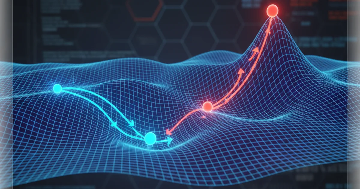
Visual comparison of Gradient Descent (minimizing) and Gradient Ascent (maximizing) on a 2D function.