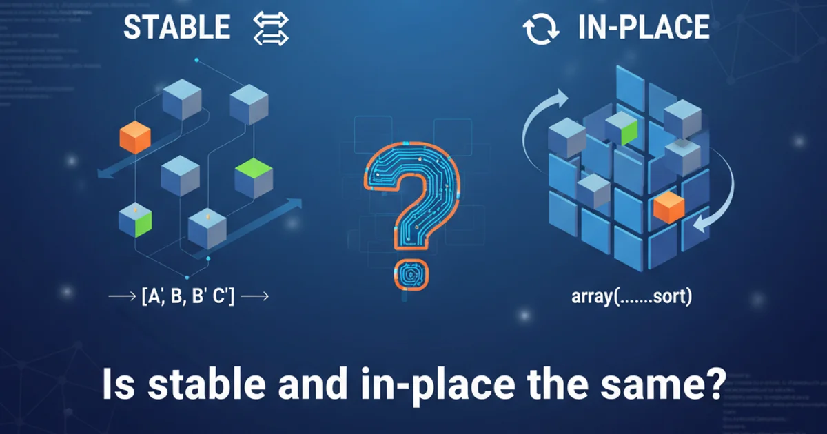
Is stable and in-place the same?
Categories:
Sorting Algorithms: Understanding Stable vs. In-Place
Explore the fundamental differences between stable and in-place sorting algorithms, their implications for data integrity and memory usage, and how to identify them.
When discussing sorting algorithms, two common terms often arise: stable and in-place. While they describe distinct characteristics, they are frequently confused or assumed to be interchangeable. This article will clarify what each term means, why these properties matter, and how they influence the choice of sorting algorithm for different applications.
What is a Stable Sorting Algorithm?
A sorting algorithm is considered stable if it preserves the relative order of equal elements. This means if two elements have the same value, their original order in the input array remains unchanged in the sorted output. Stability is crucial when elements have associated data that isn't part of the sorting key, and maintaining the original order of these equal elements is important.
flowchart TD
    A[Original Array] --> B{Sort Algorithm}
    B --> C[Sorted Array]

    subgraph Original Array
        OA1["(A, 1)"]
        OA2["(B, 2)"]
        OA3["(A, 3)"]
        OA4["(C, 4)"]
    end

    subgraph Sorted Array (Stable)
        SA1["(A, 1)"]
        SA2["(A, 3)"]
        SA3["(B, 2)"]
        SA4["(C, 4)"]
    end

    subgraph Sorted Array (Unstable)
        USA1["(A, 3)"]
        USA2["(A, 1)"]
        USA3["(B, 2)"]
        USA4["(C, 4)"]
    end

    OA1 -- "Value A, Original Index 1" --> SA1
    OA3 -- "Value A, Original Index 3" --> SA2
    OA1 -- "Value A, Original Index 1" --> USA2
    OA3 -- "Value A, Original Index 3" --> USA1

    style SA1 fill:#f9f,stroke:#333,stroke-width:2px
    style SA2 fill:#f9f,stroke:#333,stroke-width:2px
    style USA1 fill:#f9f,stroke:#333,stroke-width:2px
    style USA2 fill:#f9f,stroke:#333,stroke-width:2px

    linkStyle 0,1,2,3,4,5,6,7,8,9,10,11 stroke-width:2px,fill:none,stroke:black;
    linkStyle 12,13,14,15 stroke-width:2px,fill:none,stroke:red;
    linkStyle 16,17,18,19 stroke-width:2px,fill:none,stroke:blue;

    B -- "Stable Sort" --> SA1
    B -- "Unstable Sort" --> USA1
Comparison of stable vs. unstable sorting for elements with equal values. Notice how (A,1) and (A,3) maintain their relative order in the stable sort, but not in the unstable one.
Consider a list of students, each with a name and an ID. If you sort them by name, and then by ID, a stable sort ensures that students with the same name retain their original order based on their IDs. If the sort were unstable, the relative order of students with identical names might be arbitrarily changed.
What is an In-Place Sorting Algorithm?
An algorithm is considered in-place if it transforms the input data using only a small, constant amount of extra memory space, typically O(1) or O(log n) for recursion stack space, beyond the input itself. This means the algorithm sorts the elements directly within the original array, without needing to create a large auxiliary data structure or a copy of the array.
flowchart TD
    A[Input Array] --> B{In-Place Sort}
    B --> C[Sorted Array]

    subgraph Memory Space
        M1[Original Array Data]
        M2[O(1) Extra Space]
    end

    B -- "Modifies M1 directly" --> M1
    M1 -- "Result is C" --> C

    style M1 fill:#ccf,stroke:#333,stroke-width:2px
    style M2 fill:#fcf,stroke:#333,stroke-width:2px
An in-place sorting algorithm operates directly on the input array, requiring only a minimal amount of additional memory.
The primary advantage of in-place algorithms is their memory efficiency. This is particularly important when dealing with very large datasets where creating a copy of the data would be impractical or impossible due to memory constraints. However, achieving in-place sorting can sometimes come at the cost of increased time complexity or algorithm complexity.
Are Stable and In-Place the Same? No!
It's a common misconception that stable and in-place are related or mutually exclusive. They are entirely independent properties. An algorithm can be:
- Stable and In-Place: E.g., Insertion Sort, Bubble Sort.
- Stable but Not In-Place: E.g., Merge Sort (typically requires O(n) extra space for merging).
- Not Stable but In-Place: E.g., Heap Sort, Quick Sort (average case).
- Not Stable and Not In-Place: E.g., Some variants of Radix Sort that use auxiliary arrays.
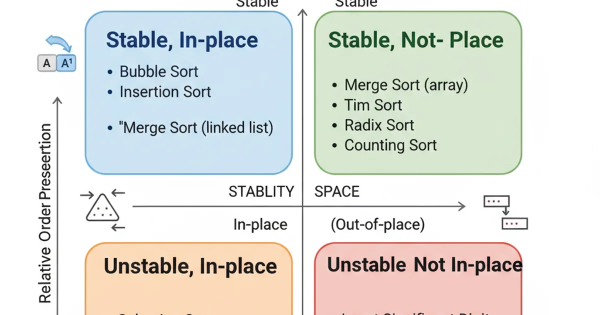
The four possible combinations of stability and in-place properties in sorting algorithms.
Why Do These Properties Matter?
The choice between stable/unstable and in-place/not-in-place algorithms depends heavily on the specific requirements of your application:
- Data Integrity (Stability): If the relative order of equal elements carries semantic meaning (e.g., preserving the original entry order for items with the same priority), then a stable sort is essential. Database systems and multi-key sorting often rely on stability.
- Memory Constraints (In-Place): For very large datasets or environments with limited memory (like embedded systems), an in-place algorithm is highly desirable to avoid out-of-memory errors or excessive swapping.
- Performance: Sometimes, achieving stability or in-place behavior can impact the time complexity. For instance, making Merge Sort in-place is possible but significantly more complex and often slower than its out-of-place variant.
std::sort in C++ or Arrays.sort for primitives in Java) are often optimized for speed and might not be stable, or their stability might depend on the data type. Always check the documentation if stability is a requirement.Understanding these distinctions allows developers to make informed decisions, balancing memory usage, performance, and data integrity requirements when implementing or choosing sorting algorithms.