How to calculate C-SCAN algorithm?

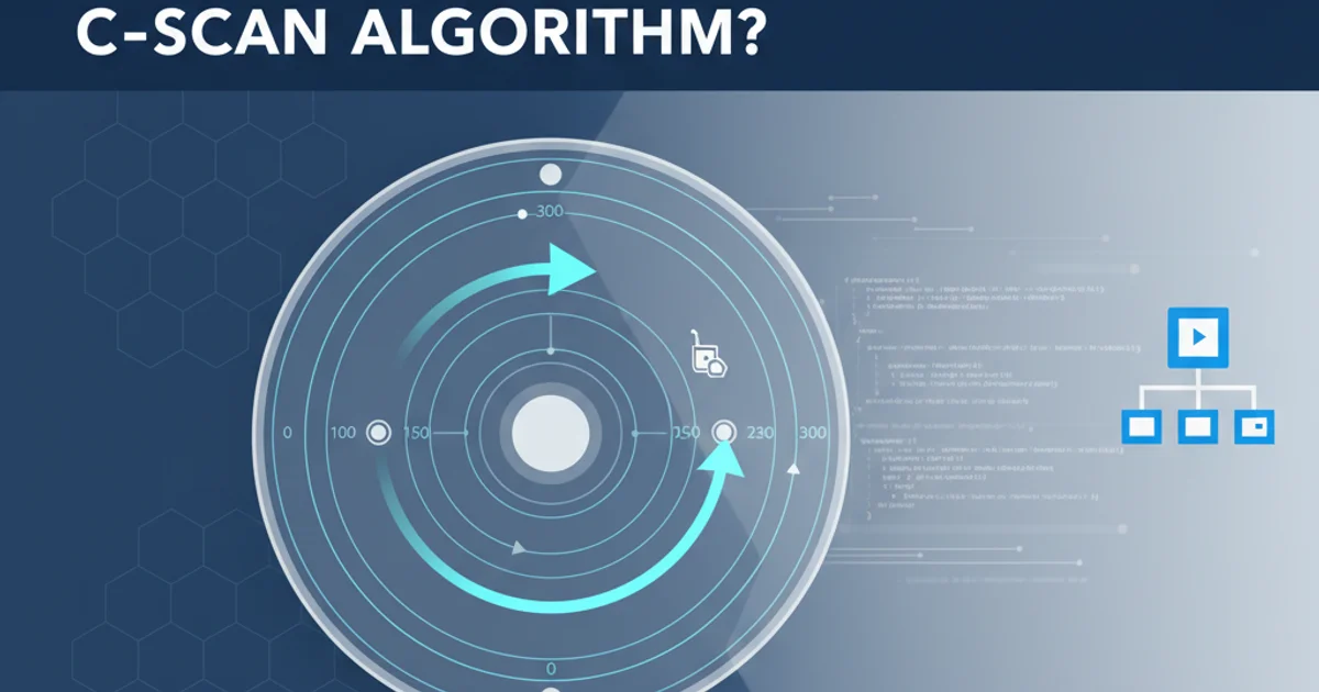
Understanding and Implementing the C-SCAN Disk Scheduling Algorithm

Explore the C-SCAN (Circular SCAN) disk scheduling algorithm, a method for optimizing disk head movement in operating systems. Learn its principles, how it works, and its advantages.

Disk scheduling algorithms are crucial components of operating systems, designed to minimize the total seek time of the disk arm. By efficiently ordering I/O requests, these algorithms improve system performance and reduce latency. Among the various strategies, C-SCAN (Circular SCAN) stands out for its fairness and predictable performance, especially in systems with heavy disk I/O.

This article will delve into the mechanics of the C-SCAN algorithm, providing a clear explanation of its operation, a step-by-step calculation example, and a visual representation using a Mermaid diagram. We'll also discuss its advantages and disadvantages compared to other scheduling methods.

What is the C-SCAN Algorithm?

The C-SCAN (Circular SCAN) algorithm is a modified version of the SCAN (Elevator) algorithm. While SCAN moves the disk arm from one end of the disk to the other, servicing requests along the way, and then reverses direction, C-SCAN operates in a strictly one-directional manner. It moves the disk arm from one end of the disk to the other, servicing all requests in its path. Once it reaches the end, it immediately returns to the beginning of the disk without servicing any requests on the return trip. After reaching the beginning, it resumes its one-directional scan, servicing requests again.

This 'circular' movement ensures that all requests receive service, and it prevents starvation, where requests at one end of the disk might wait indefinitely if new requests keep arriving at the other end. C-SCAN provides a more uniform wait time compared to SCAN, making it suitable for systems where fairness is a priority.

flowchart LR
    Start[Disk Head at Current Position] --> MoveRight{Move towards one end (e.g., highest track)}
    MoveRight --> ServiceRequests[Service requests in path]
    ServiceRequests --> EndReached{End of disk reached?}
    EndReached -- Yes --> ReturnToStart[Return to other end (e.g., lowest track) WITHOUT servicing]
    ReturnToStart --> MoveRight

Conceptual flow of the C-SCAN disk scheduling algorithm

Calculating Disk Head Movement with C-SCAN

To calculate the total head movement for C-SCAN, we need to consider the current head position, the queue of pending requests, and the total range of disk tracks. The algorithm will move in one direction, service requests, reach the end, jump to the other end, and then continue servicing requests in the same direction.

Let's consider an example:

• Disk tracks: 0 to 199
• Current head position: 53
• Request queue: 98, 183, 37, 122, 14, 124, 65, 67
• Direction: Moving towards higher track numbers (199)

1. Sort Requests and Determine Direction

First, sort the requests in ascending order: 14, 37, 65, 67, 98, 122, 124, 183. Since the head is currently at 53 and moving towards 199, it will first service requests greater than or equal to 53.

2. Scan Towards the End

The head moves from 53 towards 199, servicing requests: 53 -> 65 -> 67 -> 98 -> 122 -> 124 -> 183. The movement for this phase is (199 - 53) = 146.

3. Reach the End and Jump to Beginning

After servicing 183, the head reaches the end of the disk at 199. From 199, it jumps to the beginning of the disk at 0. The movement for this jump is (199 - 0) = 199.

4. Continue Scan from Beginning

From track 0, the head continues its scan towards 199, servicing the remaining requests: 0 -> 14 -> 37. The movement for this phase is (37 - 0) = 37.

5. Calculate Total Head Movement

Sum up all the movements: 146 (53 to 199) + 199 (199 to 0) + 37 (0 to 37) = 382 total cylinders moved.

Advantages and Disadvantages of C-SCAN

C-SCAN offers several benefits over simpler algorithms but also has its drawbacks:

Advantages:

• Fairness: Provides a more uniform wait time for requests across the disk, preventing starvation. Requests at the far end of the disk will eventually be serviced without excessive delay.
• Predictable Performance: The one-directional sweep and immediate return make its behavior more predictable than SCAN, which can change direction based on request distribution.
• Reduced Variance in Response Time: Due to its systematic approach, the variance in response times for different requests is generally lower.

Disadvantages:

• Higher Total Head Movement (Potentially): The forced sweep to the end of the disk and the immediate jump back to the beginning, even if there are no requests at the far end, can lead to higher total head movement compared to algorithms like SSTF (Shortest Seek Time First) or even SCAN in some scenarios.
• Unserviced Return Trip: The return trip from one end to the other is unproductive in terms of servicing requests, which is an overhead.
• Complexity: Slightly more complex to implement than FCFS (First-Come, First-Served) but generally simpler than algorithms requiring look-ahead or complex data structures.

def c_scan(tracks, head, requests):
    requests.sort()
    total_movement = 0
    current_head = head
    
    # Assuming disk range is 0 to max_track
    max_track = max(tracks)
    min_track = min(tracks)

    # Separate requests into two lists based on current head direction
    left_requests = [r for r in requests if r < current_head]
    right_requests = [r for r in requests if r >= current_head]

    # Move towards the right end
    for req in right_requests:
        total_movement += abs(req - current_head)
        current_head = req

    # If there are requests to the left, move to the end of the disk and then to the beginning
    if left_requests:
        # Move from current_head to max_track
        total_movement += abs(max_track - current_head)
        current_head = max_track
        
        # Jump from max_track to min_track
        total_movement += abs(max_track - min_track)
        current_head = min_track

        # Move from min_track to service remaining left requests
        for req in left_requests:
            total_movement += abs(req - current_head)
            current_head = req

    return total_movement

# Example Usage:
disk_tracks = list(range(200)) # Tracks from 0 to 199
initial_head_position = 53
request_queue = [98, 183, 37, 122, 14, 124, 65, 67]

# To simulate C-SCAN correctly, we need to adjust the logic slightly
# The standard C-SCAN moves to one end, then jumps to the other and sweeps again.
# Let's re-implement for clarity based on the example's direction (towards higher tracks first)

def calculate_c_scan_movement(current_head, requests, max_track, min_track=0):
    requests.sort()
    total_movement = 0
    path = [current_head]

    # Requests to the right (or equal) of the current head
    right_side_requests = [r for r in requests if r >= current_head]
    # Requests to the left of the current head
    left_side_requests = [r for r in requests if r < current_head]

    # 1. Move right, servicing requests
    for req in right_side_requests:
        total_movement += abs(req - current_head)
        current_head = req
        path.append(current_head)

    # 2. Move to the end of the disk (max_track)
    if current_head != max_track:
        total_movement += abs(max_track - current_head)
        current_head = max_track
        path.append(current_head)

    # 3. Jump to the beginning of the disk (min_track) without servicing
    total_movement += abs(max_track - min_track) # This is the 'jump' cost
    current_head = min_track
    path.append(current_head)

    # 4. Move right again, servicing remaining requests (which are now to the right of min_track)
    for req in left_side_requests:
        total_movement += abs(req - current_head)
        current_head = req
        path.append(current_head)

    return total_movement, path

# Using the example values:
max_disk_track = 199
movement, sequence = calculate_c_scan_movement(initial_head_position, request_queue, max_disk_track)

print(f"C-SCAN Total Head Movement: {movement}")
print(f"C-SCAN Sequence: {sequence}")

# Expected output for the example:
# C-SCAN Total Head Movement: 382
# C-SCAN Sequence: [53, 65, 67, 98, 122, 124, 183, 199, 0, 14, 37]

Python implementation of the C-SCAN algorithm calculation.