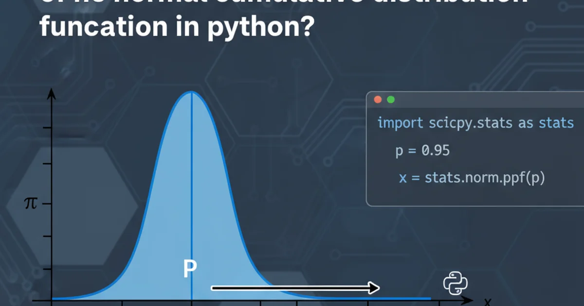
How to calculate the inverse of the normal cumulative distribution function in python?

Calculating the Inverse CDF of a Normal Distribution in Python

Learn how to efficiently compute the inverse of the normal cumulative distribution function (also known as the quantile function or probit function) in Python using the SciPy library.

The inverse of the normal cumulative distribution function (CDF), often called the quantile function or probit function, is a crucial tool in statistics and data science. It allows you to find the value (quantile) below which a given percentage of observations fall, assuming a normal distribution. For example, if you want to find the score that separates the top 5% of students, you would use the inverse CDF. Python's SciPy library provides robust and efficient methods to perform this calculation.

Understanding the Normal CDF and its Inverse

The normal CDF, denoted as ( \Phi(x) ), gives the probability that a random variable ( X ) from a normal distribution with mean ( \mu ) and standard deviation ( \sigma ) will be less than or equal to ( x ). Mathematically, it's defined as:

[ \Phi(x) = P(X \le x) = \frac{1}{\sigma\sqrt{2\pi}} \int_{-\infty}^{x} e^{-\frac{(t-\mu)^2}{2\sigma^2}} dt ]

The inverse CDF, denoted as ( \Phi^{-1}(p) ), takes a probability ( p ) (between 0 and 1) as input and returns the value ( x ) such that ( P(X \le x) = p ). In simpler terms, it answers the question: "What value ( x ) has a cumulative probability of ( p )?" This is particularly useful for hypothesis testing, confidence interval construction, and simulating data.

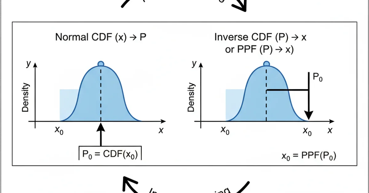
Visualizing the Normal CDF and its Inverse CDF

Using SciPy for Inverse Normal CDF

The scipy.stats module is the go-to library for statistical distributions in Python. Specifically, the norm object provides methods for the normal distribution, including its inverse CDF. The method we're interested in is ppf (percent point function), which is another name for the quantile function or inverse CDF.

from scipy.stats import norm

# Example 1: Standard Normal Distribution (mean=0, std_dev=1)
probability_standard = 0.95
quantile_standard = norm.ppf(probability_standard)
print(f"For a standard normal distribution, the value at {probability_standard*100}% cumulative probability is: {quantile_standard:.4f}")

# Example 2: Non-Standard Normal Distribution (mean=10, std_dev=2)
mean = 10
std_dev = 2
probability_non_standard = 0.025
quantile_non_standard = norm.ppf(probability_non_standard, loc=mean, scale=std_dev)
print(f"For a normal distribution (mean={mean}, std_dev={std_dev}), the value at {probability_non_standard*100}% cumulative probability is: {quantile_non_standard:.4f}")

# Example 3: Finding values for a 95% confidence interval
lower_tail_prob = 0.025 # 2.5% in the lower tail
upper_tail_prob = 0.975 # 2.5% in the upper tail (1 - 0.025)

lower_bound = norm.ppf(lower_tail_prob)
upper_bound = norm.ppf(upper_tail_prob)
print(f"For a 95% confidence interval (standard normal), the bounds are: ({lower_bound:.4f}, {upper_bound:.4f})")

Calculating inverse CDF for standard and non-standard normal distributions.

Common Applications

The inverse normal CDF has numerous practical applications across various fields:

• Statistical Inference: Determining critical values for hypothesis tests (e.g., z-scores for a given alpha level) or constructing confidence intervals.
• Risk Management: Calculating Value at Risk (VaR) in finance, which estimates the potential loss of an investment over a specific period with a given confidence level.
• Quality Control: Setting control limits for processes based on desired defect rates.
• Data Generation: Simulating normally distributed random variables from uniformly distributed random numbers (though numpy.random.normal is often preferred for direct simulation).
• Machine Learning: In some algorithms, transforming probabilities back into feature space or for inverse transformations.