Computational complexity of Inverse FFT

Understanding the Computational Complexity of Inverse FFT

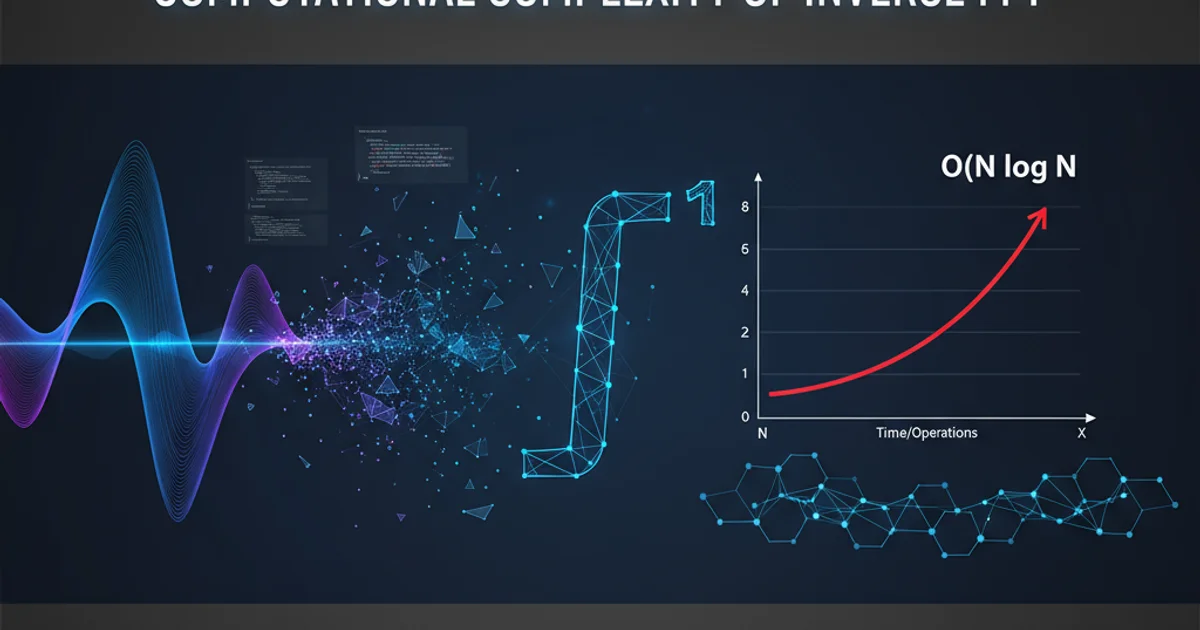
Explore the Big-O notation and computational efficiency of the Inverse Fast Fourier Transform (IFFT), a cornerstone of digital signal processing.

The Inverse Fast Fourier Transform (IFFT) is a fundamental algorithm in digital signal processing, used to convert a frequency-domain representation of a signal back into its original time-domain form. It is the inverse operation of the Fast Fourier Transform (FFT). Understanding its computational complexity is crucial for designing efficient algorithms and systems, especially when dealing with large datasets or real-time applications. This article delves into the Big-O notation of the IFFT, explaining why it shares the same efficiency as its forward counterpart.

The Relationship Between FFT and IFFT

At its core, the IFFT is remarkably similar to the FFT. In fact, an IFFT can often be computed using a standard FFT algorithm with minor modifications. The primary differences involve a conjugation of the input, a scaling factor, and potentially a conjugation of the output. This close relationship is key to understanding why their computational complexities are identical.

Consider the Discrete Fourier Transform (DFT) and its inverse (IDFT):

DFT: X_k = sum_{n=0}^{N-1} x_n * e^(-j * 2 * pi * k * n / N)

IDFT: x_n = (1/N) * sum_{k=0}^{N-1} X_k * e^(j * 2 * pi * k * n / N)

Notice the similarities: the summation structure, the exponential term, and the range of indices. The main differences are the sign in the exponent and the 1/N scaling factor for the IDFT. When these operations are optimized into their 'Fast' versions, the underlying computational structure remains largely the same.

flowchart TD
    A[Time Domain Signal x(n)] --> B{FFT Algorithm}
    B --> C[Frequency Domain Signal X(k)]
    C --> D{IFFT Algorithm}
    D --> E[Reconstructed Time Domain Signal x'(n)]
    style A fill:#f9f,stroke:#333,stroke-width:2px
    style C fill:#bbf,stroke:#333,stroke-width:2px
    style E fill:#f9f,stroke:#333,stroke-width:2px

Conceptual flow from Time Domain to Frequency Domain and back using FFT/IFFT.

Computational Complexity: O(N log N)

The computational complexity of both the FFT and IFFT is O(N log N), where N is the number of samples in the signal. This efficiency is a significant improvement over the O(N^2) complexity of the direct Discrete Fourier Transform (DFT) and Inverse Discrete Fourier Transform (IDFT).

The O(N log N) complexity arises from the 'divide and conquer' strategy employed by FFT algorithms, such as the Cooley-Tukey algorithm. This method recursively breaks down a DFT of size N into smaller DFTs. For example, a DFT of size N can be computed by combining two DFTs of size N/2. This recursive decomposition continues until the DFTs are of size 1, which are trivial to compute.

Each stage of this decomposition involves N operations (additions and multiplications), and there are log_2(N) such stages for a power-of-two N. This leads directly to the N * log_2(N) complexity. Since the IFFT essentially performs the same set of operations (just with conjugated twiddle factors and a scaling), its complexity remains identical.

Practical Implications and Performance

Understanding the O(N log N) complexity has significant practical implications:

1. Scalability: As the signal length N increases, the computation time grows much slower than N^2. This makes FFT/IFFT feasible for processing very long signals.
2. Real-time Processing: For many applications, N log N allows for real-time spectral analysis and synthesis, which would be impossible with N^2 algorithms.
3. Algorithm Choice: When implementing signal processing tasks, choosing an FFT-based approach for frequency domain operations is almost always preferred over direct DFT/IDFT calculations due to this complexity advantage.

Modern FFT/IFFT libraries are highly optimized, often leveraging hardware-specific instructions and parallel processing to achieve even greater speeds in practice. However, the theoretical O(N log N) complexity remains the fundamental benchmark.

import numpy as np
import time

def measure_complexity(N):
    # Generate a random frequency domain signal
    X = np.random.rand(N) + 1j * np.random.rand(N)

    start_time = time.time()
    x = np.fft.ifft(X)
    end_time = time.time()
    return end_time - start_time

# Test for different N values (powers of 2)
N_values = [2**i for i in range(10, 20)] # From 1024 to 524288
times = []

print("Measuring IFFT computation times:")
for N in N_values:
    t = measure_complexity(N)
    times.append(t)
    print(f"N = {N}: {t:.6f} seconds")

# You would typically plot N*log(N) vs N^2 to show the difference
# For this example, we just show the raw times.

Python example demonstrating IFFT computation time for varying N. Observe how the time grows slower than N^2.