Power spectrum of an image

Understanding the Power Spectrum of an Image

Explore how the Discrete Fourier Transform (DFT) reveals frequency components and directional information within an image, a fundamental concept in image processing.

The power spectrum of an image is a powerful tool in signal processing, offering insights into the frequency content and directional characteristics of an image. By transforming an image from its spatial domain to the frequency domain, we can analyze patterns, textures, and periodic structures that might not be immediately obvious in the original image. This article will guide you through the theoretical foundations and practical implementation of calculating and interpreting the power spectrum using MATLAB.

The Discrete Fourier Transform (DFT) for Images

At the heart of the power spectrum lies the Discrete Fourier Transform (DFT). For a 2D image, the DFT decomposes the image into its constituent sinusoidal components, each with a specific frequency, amplitude, and phase. The output of the 2D DFT is a complex-valued matrix, where each element represents a particular frequency component. The magnitude of these complex numbers indicates the strength of that frequency, while the phase indicates its position.

In the frequency domain, low frequencies correspond to the general structure and smooth variations in the image (e.g., large objects, background), while high frequencies correspond to fine details, edges, and sharp transitions (e.g., textures, noise). The center of the frequency domain typically represents the DC component (zero frequency), which corresponds to the average intensity of the image. Frequencies increase as you move away from the center.

flowchart TD
    A[Input Image (Spatial Domain)] --> B{2D DFT}
    B --> C[Frequency Domain (Complex Output)]
    C --> D{Magnitude Calculation}
    D --> E[Power Spectrum (Magnitude Squared)]
    E --> F{Log Scaling (for Visualization)}
    F --> G[Shift Zero-Frequency to Center]
    G --> H[Visualize Power Spectrum]
    H --> I[Analyze Frequency Content & Direction]

Workflow for calculating and visualizing an image's power spectrum

Calculating the Power Spectrum in MATLAB

To calculate the power spectrum of an image in MATLAB, we typically follow these steps:

1. Load and Preprocess the Image: Convert the image to grayscale and a suitable data type (e.g., double).
2. Apply 2D DFT: Use the fft2 function to compute the 2D DFT.
3. Shift Zero-Frequency Component: The fft2 function places the zero-frequency component (DC component) at the top-left corner. For better visualization, it's common practice to shift this to the center using fftshift.
4. Calculate Magnitude: Compute the magnitude of the complex DFT output using abs().
5. Calculate Power Spectrum: The power spectrum is typically defined as the square of the magnitude. This emphasizes stronger frequency components.
6. Logarithmic Scaling: The range of values in the power spectrum can be very large. Applying a logarithmic scale (e.g., log(1 + P)) helps to visualize the weaker frequency components that would otherwise be overshadowed by the strong DC component and other dominant frequencies.

% Load an example image
img = imread('cameraman.tif');

% Convert to grayscale if it's an RGB image
if size(img, 3) == 3
    img_gray = rgb2gray(img);
else
    img_gray = img;
end

% Convert to double for FFT computation
img_double = im2double(img_gray);

% Perform 2D FFT
F = fft2(img_double);

% Shift the zero-frequency component to the center
F_shifted = fftshift(F);

% Calculate the magnitude spectrum
Magnitude_Spectrum = abs(F_shifted);

% Calculate the power spectrum (magnitude squared)
Power_Spectrum = Magnitude_Spectrum.^2;

% Apply logarithmic scaling for better visualization
Power_Spectrum_Log = log(1 + Power_Spectrum);

% Display the original image and its power spectrum
figure;
subplot(1, 2, 1);
imshow(img_gray);
title('Original Image');

subplot(1, 2, 2);
imshow(Power_Spectrum_Log, []); % Use [] for automatic scaling
title('Log-Scaled Power Spectrum');

MATLAB code to compute and display the log-scaled power spectrum of an image.

Interpreting the Power Spectrum

The power spectrum provides a visual representation of the image's frequency content:

• Center (DC Component): The brightest point at the center represents the average intensity of the image. A very bright center indicates a high average intensity.
• Brightness: Brighter regions away from the center indicate strong frequency components. For example, a strong horizontal line in the spatial domain will appear as a bright vertical line in the frequency domain (perpendicular to the spatial feature).
• Directionality: Patterns in the power spectrum reveal dominant orientations in the image. If an image has many horizontal edges, the power spectrum will show strong vertical components. Conversely, vertical edges produce horizontal components.
• High vs. Low Frequencies: Frequencies close to the center are low frequencies (smooth variations), while those further out are high frequencies (sharp details, edges, noise). A spectrum with significant energy spread towards the edges suggests a noisy or highly detailed image. A spectrum concentrated near the center indicates a smooth image with fewer sharp details.

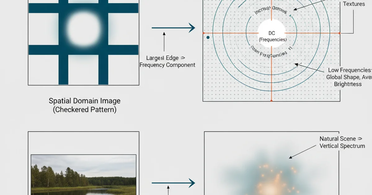
Mapping of spatial domain features to their corresponding frequency domain representations.