Convolution Vs Correlation

Convolution vs. Correlation: Understanding Key Signal Processing Operations

Explore the fundamental differences and applications of convolution and correlation in signal and image processing, with practical examples and visual explanations.

In the realms of signal processing, image processing, and even statistics, convolution and correlation are two ubiquitous mathematical operations. While often discussed together due to their similar mathematical forms, they serve distinct purposes and yield different insights. Understanding their nuances is crucial for anyone working with data analysis, filter design, or pattern recognition. This article will demystify these concepts, highlight their differences, and provide practical examples.

What is Convolution?

Convolution is a mathematical operation on two functions (f and g) that produces a third function, expressing how the shape of one is modified by the other. It's often described as a 'weighted average' or 'smoothing' operation. In signal processing, convolution is used to describe the output of a linear time-invariant (LTI) system when given an input signal and the system's impulse response. In image processing, it's fundamental to filtering operations like blurring, sharpening, and edge detection.

flowchart TD
    A[Input Signal/Image] --> B{Apply Kernel/Filter}
    B --> C[Slide Kernel Across Input]
    C --> D{Multiply & Sum at Each Position}
    D --> E[Output Signal/Image (Convolved Result)]

Conceptual flow of a convolution operation.

The mathematical definition of discrete convolution for two sequences, f[n] and g[n], is given by:

(f * g)[n] = Σ f[k] * g[n - k]

where the sum is over all possible values of k. The key aspect here is the 'flipping' or 'reversal' of the second function, g[n], before it's shifted and multiplied. This reversal is what distinguishes convolution from correlation.

import numpy as np

def convolve_1d(signal, kernel):
    output = np.zeros(signal.shape[0] + kernel.shape[0] - 1)
    # Flip the kernel for convolution
    flipped_kernel = kernel[::-1]
    for i in range(output.shape[0]):
        for j in range(kernel.shape[0]):
            if 0 <= i - j < signal.shape[0]:
                output[i] += signal[i - j] * flipped_kernel[j]
    return output

# Example usage:
signal = np.array([1, 2, 3, 4, 5])
kernel = np.array([0.5, 1, 0.5]) # A simple smoothing kernel
convolved_signal = convolve_1d(signal, kernel)
print(f"Signal: {signal}")
print(f"Kernel: {kernel}")
print(f"Convolved Signal: {convolved_signal}")

What is Correlation?

Correlation, specifically cross-correlation, measures the similarity of two signals as a function of the displacement of one relative to the other. It's used to find features in an unknown signal by comparing it to a known signal, or to detect the presence of a specific pattern within a larger signal. Unlike convolution, the second function (often called the 'template' or 'kernel') is not flipped before the multiplication and summation.

flowchart TD
    A[Input Signal/Image] --> B{Template/Pattern}
    B --> C[Slide Template Across Input]
    C --> D{Multiply & Sum at Each Position}
    D --> E[Output Signal/Image (Correlation Result)]

Conceptual flow of a correlation operation.

The mathematical definition of discrete cross-correlation for two sequences, f[n] and g[n], is given by:

(f ★ g)[n] = Σ f[k] * g[k - n]

Notice the absence of the n - k term in g's index, which signifies no flipping. This makes correlation ideal for pattern matching, as you're directly comparing the template's shape to segments of the input signal.

import numpy as np

def correlate_1d(signal, template):
    output = np.zeros(signal.shape[0] + template.shape[0] - 1)
    for i in range(output.shape[0]):
        for j in range(template.shape[0]):
            if 0 <= i - j < signal.shape[0]:
                # No flipping of the template for correlation
                output[i] += signal[i - j] * template[j]
    return output

# Example usage:
signal = np.array([0, 0, 1, 2, 3, 2, 1, 0, 0])
template = np.array([1, 2, 1]) # A pattern to search for
correlated_signal = correlate_1d(signal, template)
print(f"Signal: {signal}")
print(f"Template: {template}")
print(f"Correlated Signal: {correlated_signal}")
# The peak in correlated_signal indicates where the template best matches the signal.

Key Differences and Applications

The primary distinction between convolution and correlation lies in the 'flipping' of one of the functions. This seemingly small difference leads to vastly different applications.

• Convolution (Flipping): Used for filtering, blurring, sharpening, edge detection, and modeling linear systems. It describes how an input signal is transformed by a system's impulse response.
• Correlation (No Flipping): Used for pattern matching, template matching, time delay estimation, and feature detection. It quantifies the similarity between two signals at various shifts.

In many practical scenarios, especially with symmetric kernels (e.g., Gaussian blur), convolution and correlation yield identical results because flipping a symmetric kernel doesn't change its form. However, for asymmetric kernels, the results will differ significantly.

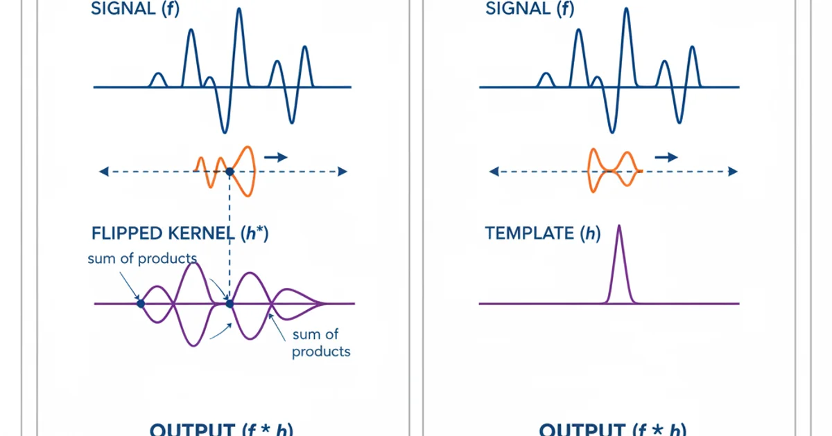
Visualizing the difference: Convolution (left) flips the kernel, while Correlation (right) does not.

Understanding when to use each operation is critical. If you're trying to modify a signal or image based on a system's characteristics (like applying a filter), convolution is your tool. If you're searching for a specific pattern or measuring similarity, correlation is more appropriate.