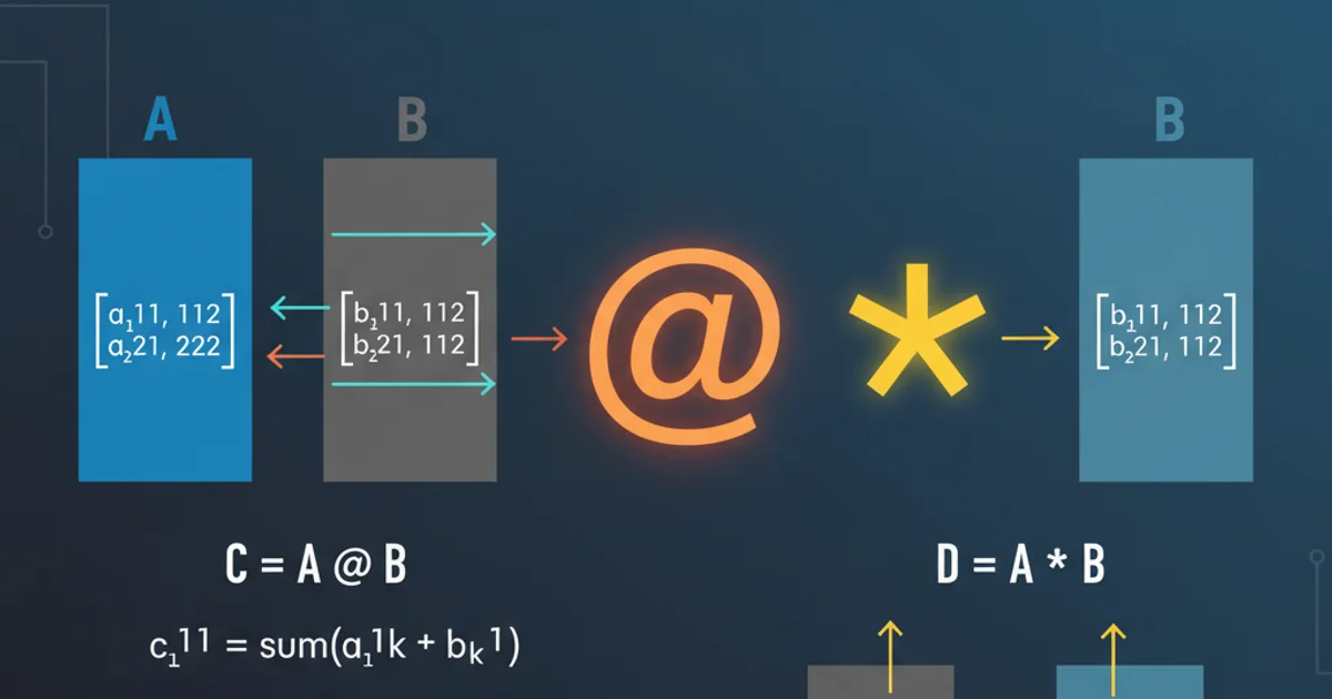
What's the difference between @ and * with python matrix multiplication?

Python Matrix Multiplication: Understanding @ vs. *

Explore the fundamental differences between the @ operator and the * operator in Python for matrix multiplication, focusing on NumPy arrays.

In Python, especially when working with numerical libraries like NumPy, understanding the distinction between the @ operator and the * operator for multiplication is crucial. While both perform multiplication, they represent entirely different mathematical operations when applied to arrays or matrices. This article will clarify these differences, provide practical examples, and help you choose the correct operator for your matrix computations.

Element-wise Multiplication with * (Hadamard Product)

The * operator in Python, when used with NumPy arrays, performs element-wise multiplication. This means that each element in the first array is multiplied by the corresponding element in the second array. For this operation to be valid, the two arrays must have compatible shapes (either identical shapes or one must be broadcastable to the other's shape). The result is an array of the same shape as the input (or the broadcasted shape).

import numpy as np

A = np.array([[1, 2], [3, 4]])
B = np.array([[5, 6], [7, 8]])

# Element-wise multiplication
C = A * B
print("Element-wise multiplication (A * B):\n", C)

Example of element-wise multiplication using the * operator.

Matrix Multiplication with @ (Dot Product)

The @ operator, introduced in Python 3.5 (PEP 465), is specifically designed for matrix multiplication (also known as the dot product). This operation follows the rules of linear algebra: the number of columns in the first matrix must equal the number of rows in the second matrix. The resulting matrix will have the number of rows from the first matrix and the number of columns from the second matrix.

import numpy as np

A = np.array([[1, 2], [3, 4]])
B = np.array([[5, 6], [7, 8]])

# Matrix multiplication
D = A @ B
print("Matrix multiplication (A @ B):\n", D)

# Example with incompatible shapes for matrix multiplication
E = np.array([[1, 2, 3], [4, 5, 6]]) # 2x3 matrix
F = np.array([[7, 8], [9, 10]])    # 2x2 matrix

# This would raise a ValueError: 'matmul: Input operand 1 has a mismatch in its core dimension 0, with gufunc signature (n?,k),(k,m?)->(n?,m?) (inferred 2 vs. 3)'
# try:
#     G = E @ F
# except ValueError as e:
#     print(f"\nError for E @ F: {e}")

# Corrected example for matrix multiplication
F_compatible = np.array([[7, 8], [9, 10], [11, 12]]) # 3x2 matrix
H = E @ F_compatible
print("\nMatrix multiplication (E @ F_compatible):\n", H)

Example of matrix multiplication using the @ operator, including a demonstration of shape compatibility.

Visualizing the Operations

To further clarify the distinction, let's visualize how these operations work with two simple 2x2 matrices. This diagram illustrates the flow of data for both element-wise and matrix multiplication.

flowchart LR
    subgraph Input Matrices
        A["Matrix A (2x2)"]
        B["Matrix B (2x2)"]
    end

    A -- "Element-wise (A * B)" --> C[["Result C (2x2)"]]
    C -- "(A[i,j] * B[i,j])" --> C_detail("e.g., C[0,0] = A[0,0] * B[0,0]")

    A -- "Matrix Multiplication (A @ B)" --> D[["Result D (2x2)"]]
    D -- "(Sum of products of rows and columns)" --> D_detail("e.g., D[0,0] = A[0,0]*B[0,0] + A[0,1]*B[1,0]")

    style C fill:#e0ffe0,stroke:#333,stroke-width:2px
    style D fill:#e0e0ff,stroke:#333,stroke-width:2px

Comparison of element-wise (*) vs. matrix (@) multiplication.

When to Use Which Operator

Choosing between * and @ depends entirely on the mathematical operation you intend to perform:

• Use * for element-wise operations: When you need to multiply corresponding elements of two arrays. This is common in statistical calculations, image processing (e.g., applying masks), or when scaling data.
• Use @ for matrix multiplication: When you are performing linear algebra operations, such as transforming vectors, solving systems of linear equations, or implementing neural networks. This is the standard mathematical definition of matrix product.

It's important to note that for scalar multiplication (multiplying an array by a single number), both * and @ will behave similarly by performing element-wise multiplication. However, it's best practice to use * for scalar multiplication to maintain clarity and consistency.

import numpy as np

A = np.array([[1, 2], [3, 4]])
scalar = 5

# Scalar multiplication using *
result_star = A * scalar
print("Scalar multiplication (A * scalar):\n", result_star)

# Scalar multiplication using @ (behaves similarly, but * is preferred)
result_at = A @ scalar
print("Scalar multiplication (A @ scalar):\n", result_at)

Scalar multiplication with * and @.