Calculating a p-value for the spearman's rank statistic in excel (using vba or not)

Calculating Spearman's Rank Correlation P-Value in Excel (with/without VBA)

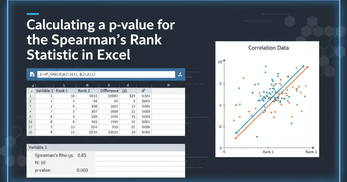
Learn how to compute the p-value for Spearman's rank correlation coefficient in Excel, covering both manual formula-based approaches and automated VBA solutions for statistical significance.

Spearman's rank correlation coefficient (ρ) is a non-parametric measure of the strength and direction of association between two ranked variables. While Excel can easily calculate the coefficient itself, determining the statistical significance (p-value) often requires additional steps. This article will guide you through calculating the p-value for Spearman's ρ in Excel, offering both formula-based methods and a VBA solution for greater automation.

Understanding Spearman's Rank Correlation and P-Value

Before diving into calculations, it's crucial to understand what Spearman's ρ and its associated p-value represent. Spearman's ρ assesses how well the relationship between two variables can be described using a monotonic function. A monotonic function is one that is either entirely non-increasing or entirely non-decreasing. Unlike Pearson's correlation, Spearman's does not require the data to be normally distributed or the relationship to be linear.

The p-value, on the other hand, helps us determine the statistical significance of the observed correlation. It represents the probability of observing a correlation as extreme as, or more extreme than, the one calculated, assuming that there is no actual correlation in the population (the null hypothesis). A small p-value (typically < 0.05) suggests that the observed correlation is unlikely to have occurred by chance, leading us to reject the null hypothesis and conclude that a significant monotonic relationship exists.

flowchart TD
    A[Start with Raw Data] --> B{Rank Data for X and Y}
    B --> C[Calculate Difference in Ranks (d)]
    C --> D[Square Differences (d^2)]
    D --> E[Sum Squared Differences (Σd^2)]
    E --> F[Calculate Spearman's ρ]
    F --> G{Determine Sample Size (n)}
    G --> H[Calculate t-statistic (for n > 10)]
    H --> I[Calculate Degrees of Freedom (df = n-2)]
    I --> J[Find P-value using T.DIST.2T]
    F --> K{For n <= 10, use critical values table}
    K --> L[Compare ρ with Critical Value]
    L --> M[Determine Significance]
    J --> M[Determine Significance]
    M --> N[End]

Flowchart for Calculating Spearman's P-Value

Method 1: Manual Calculation in Excel (Formulas)

This method involves several steps within Excel using built-in functions. It's suitable for smaller datasets or when you need to see each step of the calculation.

Step 1: Rank Your Data

First, you need to rank your independent (X) and dependent (Y) variables. If there are ties, assign the average rank to the tied values. Excel's RANK.AVG function is perfect for this.

Let's assume your X data is in A2:A11 and Y data is in B2:B11.

• In cell C2, enter =RANK.AVG(A2,$A$2:$A$11,1) and drag down.
• In cell D2, enter =RANK.AVG(B2,$B$2:$B$11,1) and drag down.

Step 2: Calculate Differences in Ranks (d) and Squared Differences (d²)

• In cell E2, enter =C2-D2 (difference in ranks) and drag down.
• In cell F2, enter =E2^2 (squared difference) and drag down.

Step 3: Sum the Squared Differences (Σd²)

• In cell F12 (or any empty cell below), enter =SUM(F2:F11).

Step 4: Calculate Spearman's Rank Correlation Coefficient (ρ)

The formula for Spearman's ρ is:

ρ = 1 - (6 * Σd²) / (n * (n² - 1))

Where:

• n is the number of data pairs.

• Σd² is the sum of the squared differences in ranks.

• In cell G2, enter the number of pairs (e.g., 10).

• In cell G3, enter the formula for ρ: =1 - (6 * F12) / (G2 * (G2^2 - 1))

Step 5: Calculate the P-Value (for n > 10)

For sample sizes n > 10, we can approximate the p-value using a t-distribution. The test statistic t is calculated as:

t = ρ * sqrt((n - 2) / (1 - ρ²))

• In cell G4, calculate t: =G3 * SQRT((G2 - 2) / (1 - G3^2))
• In cell G5, calculate the p-value using Excel's T.DIST.2T function (two-tailed test): =T.DIST.2T(ABS(G4), G2 - 2)

ABS(G4) is used because the t-distribution function requires a positive value, and G2 - 2 is the degrees of freedom.

Method 2: Automated P-Value Calculation with VBA

For repetitive tasks or larger datasets, a VBA function can streamline the process of calculating Spearman's ρ and its p-value. This custom function will take two ranges as input and return the p-value directly.

Step 1: Open the VBA Editor

Press Alt + F11 to open the VBA editor.

Step 2: Insert a New Module

In the VBA editor, go to Insert > Module.

Step 3: Paste the VBA Code

Paste the following VBA code into the new module.

Function SpearmanPValue(Range1 As Range, Range2 As Range) As Double
    Dim n As Long
    Dim i As Long
    Dim d As Double
    Dim sum_d_squared As Double
    Dim rho As Double
    Dim t_stat As Double
    Dim p_val As Double
    
    ' Ensure ranges are of the same size
    If Range1.Cells.Count <> Range2.Cells.Count Then
        SpearmanPValue = CVErr(xlErrValue)
        Exit Function
    End If
    
    n = Range1.Cells.Count
    If n < 3 Then ' Need at least 3 data points for correlation
        SpearmanPValue = CVErr(xlErrValue)
        Exit Function
    End If
    
    ' Create arrays for ranks
    Dim ranks1() As Double
    Dim ranks2() As Double
    ReDim ranks1(1 To n)
    ReDim ranks2(1 To n)
    
    ' Populate ranks using Excel's RANK.AVG function
    For i = 1 To n
        ranks1(i) = Application.WorksheetFunction.Rank_Avg(Range1.Cells(i).Value, Range1, 1)
        ranks2(i) = Application.WorksheetFunction.Rank_Avg(Range2.Cells(i).Value, Range2, 1)
    Next i
    
    ' Calculate sum of squared differences in ranks
    sum_d_squared = 0
    For i = 1 To n
        d = ranks1(i) - ranks2(i)
        sum_d_squared = sum_d_squared + (d * d)
    Next i
    
    ' Calculate Spearman's Rho
    rho = 1 - (6 * sum_d_squared) / (n * (n * n - 1))
    
    ' Calculate p-value using t-distribution approximation for n > 10
    If n > 10 Then
        ' Handle perfect correlation (rho = 1 or -1) to avoid division by zero or log of zero
        If Abs(rho) = 1 Then
            p_val = 0 ' Perfect correlation is highly significant
        Else
            t_stat = rho * Sqr((n - 2) / (1 - (rho * rho)))
            p_val = Application.WorksheetFunction.T_Dist_2T(Abs(t_stat), n - 2)
        End If
    Else
        ' For n <= 10, approximation is not reliable. Return a specific error or indicator.
        ' In a real scenario, you'd compare rho to critical values from a table.
        ' For simplicity, we'll return a placeholder or indicate manual check needed.
        ' Here, we'll return -1 to indicate 'manual check needed' or 'not applicable'.
        ' A more robust solution might involve embedding critical values or a lookup.
        p_val = -1 ' Indicates manual check needed for small n
    End If
    
    SpearmanPValue = p_val
End Function

VBA function to calculate Spearman's P-Value

Using the VBA Function

After pasting the VBA code, you can use the SpearmanPValue function directly in your Excel worksheet like any other built-in function.

Assuming your X data is in A2:A11 and Y data is in B2:B11:

• In any empty cell, enter =SpearmanPValue(A2:A11, B2:B11).

The function will return the p-value. If n <= 10, it will return -1, indicating that the t-distribution approximation is not suitable and a manual check against critical values is required.