How to filter in excel based on many unique values?

Efficiently Filter Excel Data by Many Unique Values

Learn advanced techniques to filter large datasets in Excel using multiple unique criteria, moving beyond basic filtering to handle complex scenarios with ease.

Filtering data in Excel is a fundamental skill, but when you need to filter by a large number of unique values, the standard AutoFilter or Advanced Filter can become cumbersome. This article explores several powerful methods to efficiently filter your Excel data based on many unique criteria, ranging from formula-based approaches to leveraging Power Query, ensuring you can tackle even the most complex filtering tasks.

The Challenge of Many Unique Values

Traditional Excel filtering methods, while effective for simple tasks, quickly become impractical when dealing with hundreds or thousands of unique values. Manually selecting checkboxes in the AutoFilter dropdown is time-consuming and prone to errors. Advanced Filter offers more flexibility but still requires careful setup, especially when your criteria list is dynamic or extensive. This section outlines why these methods fall short and introduces the need for more robust solutions.

flowchart TD
    A[Start Filtering Task] --> B{Number of Unique Values?}
    B -->|Few (e.g., <20)| C[Use AutoFilter/Basic Filter]
    B -->|Many (e.g., >20)| D{Criteria List Dynamic?}
    D -->|No| E[Use Advanced Filter with Static Range]
    D -->|Yes| F[Consider Formula-Based Filtering]
    F --> G[Consider Power Query]
    G --> H[Consider VBA Macro]
    H --> I[End Filtering Task]

Decision flow for choosing an Excel filtering method

Method 1: Formula-Based Filtering with FILTER and TOROW (Excel 365)

For users with Excel 365, dynamic array functions provide an incredibly powerful and flexible way to filter data. The FILTER function, combined with TOROW and COUNTIF or MATCH, allows you to filter a range based on a list of criteria values. This method is dynamic, meaning your filtered results update automatically when source data or criteria change.

=FILTER(A2:C100, ISNUMBER(MATCH(A2:A100, E2:E10, 0)))

Example of filtering a range (A2:C100) where values in column A match any value in the criteria list (E2:E10).

1. Prepare Your Data

Ensure your main data range is organized, and your list of unique filter criteria is in a separate column or range (e.g., E2:E10).

2. Enter the Formula

Select a cell where you want the filtered results to appear (e.g., G2). Enter the FILTER formula, adjusting ranges to match your data. The ISNUMBER(MATCH(...)) part checks if each value in your data's filter column exists in your criteria list.

3. Review Results

The filtered data will spill into adjacent cells. If your criteria list or source data changes, the results will update automatically.

Method 2: Power Query for Robust Filtering

Power Query (Get & Transform Data) is Excel's built-in ETL (Extract, Transform, Load) tool, ideal for complex data manipulation, including filtering by many unique values. It's particularly useful when dealing with external data sources, large datasets, or when you need to repeat the filtering process regularly. Power Query allows you to define a query that filters your main data based on a list of values from another table or range.

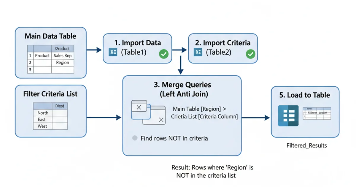
Power Query workflow for filtering data using a separate criteria list.

1. Load Data to Power Query

Convert your main data range and your criteria list into Excel Tables. Then, for each table, go to Data > Get & Transform Data > From Table/Range to load them into Power Query Editor.

2. Merge Queries

In the Power Query Editor, select your main data query. Go to Home > Combine > Merge Queries. In the Merge dialog, select your main data table and the column you want to filter by. Then select your criteria table and its column containing the unique values. Choose a 'Left Anti' or 'Inner' join type depending on whether you want to exclude or include matches.

3. Filter and Load

After merging, you'll have a new column indicating matches. Filter this column as needed (e.g., remove nulls for 'Inner' join). Finally, click Home > Close & Load To... to load the filtered results back into a new Excel sheet.

Method 3: VBA Macro for Custom Filtering Logic

For highly specific or automated filtering requirements, a VBA macro offers the ultimate flexibility. You can write code to iterate through your criteria list and apply filters programmatically. This method is best for users comfortable with VBA or when other methods don't meet unique business logic needs.

Sub FilterByManyValues()
    Dim wsData As Worksheet
    Dim wsCriteria As Worksheet
    Dim rngData As Range
    Dim rngCriteria As Range
    Dim arrCriteria() As Variant
    Dim i As Long
    Dim lastRowData As Long
    Dim lastRowCriteria As Long

    Set wsData = ThisWorkbook.Sheets("Sheet1") ' Your data sheet name
    Set wsCriteria = ThisWorkbook.Sheets("Criteria") ' Your criteria sheet name

    ' Find last row of data and criteria
    lastRowData = wsData.Cells(wsData.Rows.Count, "A").End(xlUp).Row
    lastRowCriteria = wsCriteria.Cells(wsCriteria.Rows.Count, "A").End(xlUp).Row

    ' Define data range (e.g., A1:C & lastRowData)
    Set rngData = wsData.Range("A1:C" & lastRowData)

    ' Define criteria range (e.g., A2:A & lastRowCriteria, assuming header in A1)
    Set rngCriteria = wsCriteria.Range("A2:A" & lastRowCriteria)

    ' Load criteria into an array
    If lastRowCriteria > 1 Then
        arrCriteria = Application.Transpose(rngCriteria.Value)
    Else
        MsgBox "No criteria found.", vbExclamation
        Exit Sub
    End If

    ' Apply AutoFilter
    If wsData.AutoFilterMode Then wsData.AutoFilterMode = False ' Turn off existing filter
    rngData.AutoFilter Field:=1, Criteria1:=arrCriteria, Operator:=xlFilterValues

    MsgBox "Filtering complete!", vbInformation
End Sub

VBA macro to filter data in 'Sheet1' based on a list of values in 'Criteria' sheet.