How to Create an excel dropdown list that displays text with a numeric hidden value

How to Create an Excel Dropdown List with Display Text and Hidden Numeric Values

Learn to implement Excel dropdown lists that show user-friendly text while storing corresponding numeric values, perfect for data analysis and reporting.

Excel dropdown lists are powerful tools for data entry and validation, ensuring consistency and reducing errors. However, a common challenge arises when you want users to select from a list of descriptive text options (e.g., "High", "Medium", "Low") but need to store or use a corresponding numeric value (e.g., 3, 2, 1) for calculations or analysis. This article will guide you through creating such a dropdown list, allowing you to display text while working with hidden numeric values.

Understanding the Need for Hidden Numeric Values

Imagine you're tracking project priorities. Presenting options like "High", "Medium", and "Low" is intuitive for users. However, for reporting, sorting, or weighted calculations, assigning numeric values (e.g., High=3, Medium=2, Low=1) is far more efficient. Directly using text in formulas can be cumbersome, requiring complex IF or VLOOKUP statements. By linking text to hidden numeric values, you streamline your data processing without sacrificing user experience.

flowchart TD
    A["User Selects 'High'"] --> B{"Dropdown Cell"}
    B --> C["Display 'High'"]
    C --> D["Hidden Cell (e.g., VLOOKUP)"]
    D --> E["Stores '3'"]
    E --> F["Used in Calculations/Reports"]
    A --> F

Workflow for displaying text while storing a hidden numeric value.

Setting Up Your Data Source

The core of this technique relies on a well-structured data source. You'll need a table (or range) that maps your display text to its corresponding numeric value. It's best practice to place this data on a separate sheet or a hidden part of your current sheet to keep your main data clean.

1. Create a Mapping Table

On a new worksheet (e.g., named Lists) or a dedicated range, create two columns. The first column will contain your display text (e.g., "High", "Medium", "Low"), and the second column will contain the corresponding numeric values (e.g., 3, 2, 1). Ensure the display text column is the first column in your mapping table.

2. Define a Named Range (Optional but Recommended)

Select the entire range of your mapping table (e.g., A1:B3 on your Lists sheet). Go to the 'Formulas' tab, click 'Define Name', and give it a descriptive name like PriorityMapping. This makes formulas easier to read and maintain.

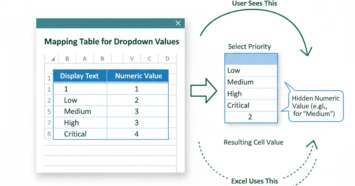
Example of a mapping table for dropdown values.

Creating the Dropdown List and Extracting the Numeric Value

Now that your data source is ready, you can create the dropdown list in your main data entry area and then use a lookup function to retrieve the associated numeric value.

1. Create the Dropdown List

Select the cell(s) where you want the dropdown list to appear. Go to the 'Data' tab, click 'Data Validation' (in the 'Data Tools' group). In the 'Data Validation' dialog box, under the 'Settings' tab:

1. Set 'Allow:' to 'List'.
2. In the 'Source:' field, enter the range of your display text column (e.g., =Lists!$A$1:$A$3 or =PriorityMapping if you defined a named range for just the display text column). Make sure to only select the display text column for the source.

2. Extract the Numeric Value

In an adjacent cell (or a cell you can hide), enter a VLOOKUP or XLOOKUP formula to retrieve the numeric value based on the selected text. If your dropdown is in cell A2 and your mapping table is Lists!A1:B3 (or named PriorityMapping), the formula would be:

=VLOOKUP(A2, Lists!A1:B3, 2, FALSE)

Or, using XLOOKUP (available in newer Excel versions):

=XLOOKUP(A2, Lists!A1:A3, Lists!B1:B3, "", FALSE)

This formula looks up the text selected in A2 within the first column of your mapping table and returns the value from the second column.

=VLOOKUP(A2, Lists!A1:B3, 2, FALSE)

VLOOKUP formula to retrieve the numeric value from a mapping table.

=XLOOKUP(A2, Lists!A1:A3, Lists!B1:B3, "", FALSE)

XLOOKUP formula (modern Excel) to retrieve the numeric value.

Advanced Considerations and Best Practices

While the basic setup is straightforward, consider these points for a more robust and user-friendly solution:

Dynamic Ranges: If your list of options might grow, convert your mapping table into an Excel Table (Insert > Table). Then, when defining your Data Validation source and VLOOKUP/XLOOKUP ranges, refer to the table columns (e.g., Table1[Display Text]). This automatically expands the ranges as you add new items.

Error Handling: Wrap your VLOOKUP or XLOOKUP formula in an IFERROR function to display a blank or a custom message if the lookup value isn't found (e.g., =IFERROR(VLOOKUP(A2, Lists!A1:B3, 2, FALSE), "")).

Conditional Formatting: You can use conditional formatting on the dropdown cell itself to highlight selections based on their underlying numeric value, providing visual cues to the user.