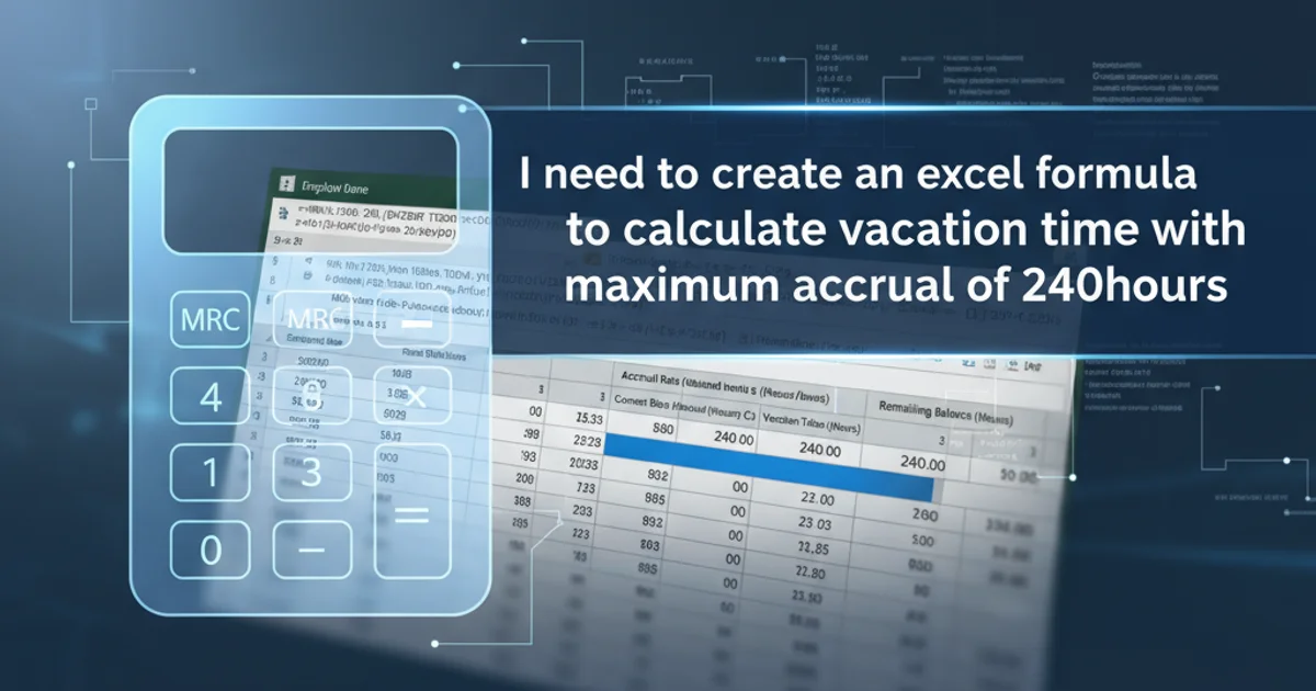
I need to create an excel formula to calculate vacation time with maximum accrual of 240hours

Mastering Excel: Calculating Vacation Accrual with a 240-Hour Cap

Learn how to create robust Excel formulas to accurately calculate employee vacation time, including a critical maximum accrual limit of 240 hours. This guide covers various scenarios and provides step-by-step instructions.

Managing employee vacation time is a common task for HR professionals and small business owners. While many dedicated software solutions exist, Microsoft Excel remains a powerful and flexible tool for tracking accruals, especially when specific rules like maximum caps are involved. This article will guide you through building an Excel formula to calculate vacation time, ensuring that no employee accrues more than 240 hours, a common policy limit.

Understanding Vacation Accrual Basics

Before diving into the formulas, it's essential to understand the core components of vacation accrual. Typically, employees accrue vacation hours based on a set rate per pay period, per month, or per year. For instance, an employee might accrue 10 hours of vacation per month. The challenge arises when a maximum accrual limit is introduced, meaning an employee cannot accumulate more than a certain number of hours, even if their regular accrual rate would push them over that limit.

flowchart TD
    A[Start Accrual Calculation] --> B{Current Accrued Hours?}
    B -->|Yes| C[Add New Accrual]
    B -->|No| D[Start with New Accrual]
    C --> E[Total Accrued = Current + New]
    D --> E
    E --> F{Total Accrued > Max Cap (240)?}
    F -->|Yes| G[Set Total Accrued = Max Cap]
    F -->|No| H[Keep Total Accrued]
    G --> I[End Calculation]
    H --> I

Vacation Accrual Logic with Maximum Cap

Setting Up Your Excel Sheet

To begin, organize your Excel sheet with the necessary columns. A typical setup might include:

• Employee Name: For identification.
• Accrual Rate: The rate at which vacation is earned (e.g., hours per pay period).
• Previous Balance: Vacation hours carried over from the last period.
• Hours Accrued This Period: The amount earned in the current cycle.
• Hours Used This Period: Vacation hours taken in the current cycle.
• Current Balance (Before Cap): The sum of previous balance + accrued - used.
• Final Balance (After Cap): The balance after applying the 240-hour maximum.

=MIN(240, B2+C2-D2)

Basic vacation accrual formula with a 240-hour cap.

Building the Core Formula with a Cap

Let's assume the following:

• B2: Represents the 'Previous Balance' (hours carried over).
• C2: Represents 'Hours Accrued This Period'.
• D2: Represents 'Hours Used This Period'.
• The maximum accrual cap is 240 hours.

The goal is to calculate the 'Final Balance' in cell E2 (or whichever column you designate).

The MIN function is perfect for applying a maximum cap. It returns the smallest number from a set of values. By comparing the calculated balance with the cap, it ensures the balance never exceeds the cap.

=MIN(240, (B2 + C2) - D2)

Detailed formula for calculating vacation balance with a 240-hour maximum.

Handling Different Accrual Scenarios

The basic formula works well, but you might encounter more complex scenarios:

Scenario 1: Accrual Rate Based on Employment Date

If the accrual rate changes based on an employee's tenure, you might need an IF or VLOOKUP function to determine the correct Hours Accrued This Period.

Scenario 2: Prorated Accrual for Partial Periods

For new hires or employees leaving mid-period, you might need to prorate the accrual. This usually involves calculating a daily accrual rate and multiplying it by the number of days worked in the period.

Scenario 3: Accrual Paused After Reaching Cap

Some policies state that accrual stops once the cap is reached, and only resumes when the balance drops below the cap. The MIN function handles this implicitly for the final balance, but if you need to show 'Hours Accrued This Period' as 0 once the cap is hit, you'd adjust the C2 value itself.

=IF(B2 >= 240, 0, [Your_Normal_Accrual_Calculation])

Formula to stop accrual if the previous balance is already at the cap.

Practical Implementation Steps

Follow these steps to implement the vacation accrual system in your Excel sheet:

1. Set up Column Headers

Create clear headers for 'Employee Name', 'Accrual Rate', 'Previous Balance', 'Hours Accrued This Period', 'Hours Used This Period', and 'Final Balance'.

2. Input Initial Data

Populate the 'Employee Name', 'Accrual Rate', and 'Previous Balance' for each employee. For new employees, 'Previous Balance' will be 0.

3. Calculate Periodic Accrual

In the 'Hours Accrued This Period' column, enter the formula to calculate the hours earned for the current period based on the employee's accrual rate. This might be a simple multiplication or a more complex IF statement.

4. Enter Hours Used

Manually input or link to another sheet for 'Hours Used This Period' for each employee.

5. Apply the Cap Formula

In the 'Final Balance' column, use the formula =MIN(240, (Previous_Balance_Cell + Accrued_This_Period_Cell) - Hours_Used_This_Period_Cell). Replace the placeholder cell references with your actual cell locations (e.g., B2, C2, D2).

6. Drag and Fill

Drag the formula down to apply it to all employees. Excel will automatically adjust cell references.

7. Review and Validate

Periodically review the calculations to ensure accuracy, especially after making changes to accrual rates or policies.