Fitting a Normal distribution to 1D data

Fitting a Normal Distribution to 1D Data in Python

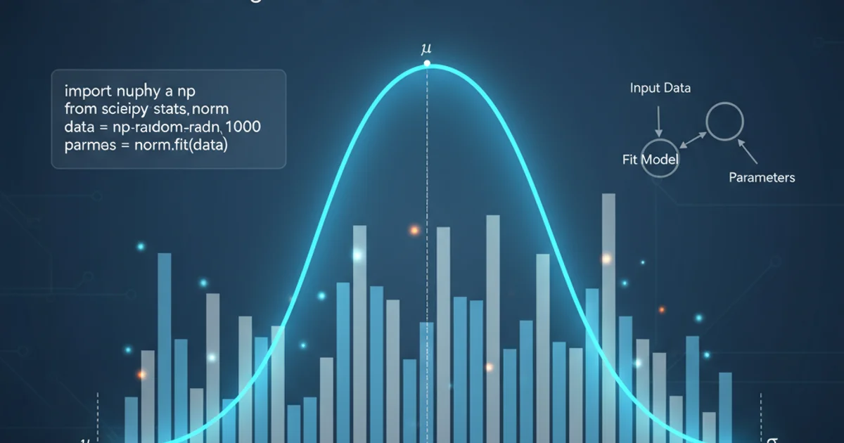
Learn how to fit a Normal (Gaussian) distribution to one-dimensional data using Python's NumPy, SciPy, and Matplotlib libraries. This guide covers estimating parameters, visualizing the fit, and understanding the underlying concepts.

Understanding the distribution of your data is a fundamental step in many data analysis tasks. The Normal distribution, also known as the Gaussian distribution or bell curve, is one of the most common and important continuous probability distributions. It's characterized by two parameters: the mean (μ) and the standard deviation (σ). This article will guide you through the process of fitting a Normal distribution to a 1D dataset using Python, covering data generation, parameter estimation, and visualization.

Generating Sample Data

Before we can fit a distribution, we need some data. For demonstration purposes, we'll generate a synthetic dataset that is approximately normally distributed. This allows us to know the true parameters and evaluate the accuracy of our fitting process. We'll use NumPy's random.normal function to create this data.

import numpy as np
import matplotlib.pyplot as plt
from scipy.stats import norm

# Parameters for our synthetic data
mu_true = 50  # True mean
sigma_true = 10 # True standard deviation
n_samples = 1000 # Number of data points

# Generate normally distributed data
data = np.random.normal(mu_true, sigma_true, n_samples)

# Plot a histogram of the generated data
plt.hist(data, bins=30, density=True, alpha=0.6, color='g', label='Histogram of Data')
plt.title('Histogram of Generated Normal Data')
plt.xlabel('Value')
plt.ylabel('Frequency')
plt.legend()
plt.grid(True)
plt.show()

Python code to generate synthetic normally distributed data and plot its histogram.

Estimating Distribution Parameters

To fit a Normal distribution, we need to estimate its mean (μ) and standard deviation (σ) from our observed data. For a Normal distribution, the maximum likelihood estimates (MLE) for these parameters are simply the sample mean and sample standard deviation. NumPy provides convenient functions for calculating these statistics.

# Estimate parameters from the data
mu_estimated = np.mean(data)
sigma_estimated = np.std(data)

print(f"Estimated Mean (μ): {mu_estimated:.2f}")
print(f"Estimated Standard Deviation (σ): {sigma_estimated:.2f}")
print(f"True Mean (μ): {mu_true}")
print(f"True Standard Deviation (σ): {sigma_true}")

Calculating the sample mean and standard deviation as estimates for the Normal distribution parameters.

Visualizing the Fitted Distribution

Once we have the estimated parameters, we can plot the probability density function (PDF) of the fitted Normal distribution alongside the histogram of our data. This visual comparison helps us assess how well the distribution fits the observed data. SciPy's norm module is excellent for this, providing functions like pdf.

# Plot the histogram again
plt.hist(data, bins=30, density=True, alpha=0.6, color='g', label='Histogram of Data')

# Plot the fitted PDF
x = np.linspace(data.min(), data.max(), 100)
p_fitted = norm.pdf(x, mu_estimated, sigma_estimated)
plt.plot(x, p_fitted, 'r-', linewidth=2, label=f'Fitted Normal PDF (μ={mu_estimated:.2f}, σ={sigma_estimated:.2f})')

plt.title('Normal Distribution Fit to 1D Data')
plt.xlabel('Value')
plt.ylabel('Probability Density')
plt.legend()
plt.grid(True)
plt.show()

Plotting the histogram of the data with the fitted Normal distribution's PDF overlaid.

flowchart TD
    A[Start: Generate Data] --> B{Calculate Sample Mean & Std Dev}
    B --> C[Estimate μ and σ]
    C --> D[Create PDF from Estimated Parameters]
    D --> E[Plot Histogram of Data]
    E --> F[Overlay Fitted PDF]
    F --> G[End: Visualize Fit]

Workflow for fitting and visualizing a Normal distribution to 1D data.

Using SciPy's norm.fit() for Convenience

SciPy provides a convenient fit() method for many distributions, including norm. This method automatically estimates the parameters (mean and standard deviation for the Normal distribution) from the data using maximum likelihood estimation. It returns the estimated parameters directly.

# Use scipy.stats.norm.fit() to get parameters
mu_scipy, sigma_scipy = norm.fit(data)

print(f"SciPy Estimated Mean (μ): {mu_scipy:.2f}")
print(f"SciPy Estimated Standard Deviation (σ): {sigma_scipy:.2f}")

# Plotting with SciPy's fit
plt.hist(data, bins=30, density=True, alpha=0.6, color='b', label='Histogram of Data')
x = np.linspace(data.min(), data.max(), 100)
p_scipy_fitted = norm.pdf(x, mu_scipy, sigma_scipy)
plt.plot(x, p_scipy_fitted, 'r--', linewidth=2, label=f'SciPy Fitted PDF (μ={mu_scipy:.2f}, σ={sigma_scipy:.2f})')

plt.title('Normal Distribution Fit using SciPy.norm.fit()')
plt.xlabel('Value')
plt.ylabel('Probability Density')
plt.legend()
plt.grid(True)
plt.show()

Fitting a Normal distribution using scipy.stats.norm.fit() and visualizing the result.