Excel: Pivot table not showing all Fields
Categories:
Excel Pivot Table Not Showing All Fields: Troubleshooting Guide
Learn why your Excel Pivot Table might not be displaying all expected fields and how to resolve common issues to ensure accurate data analysis.
Pivot Tables are powerful tools in Excel for summarizing and analyzing large datasets. However, it's a common frustration when not all of your source data fields appear in the PivotTable Fields list. This can hinder your analysis and lead to incomplete reports. This article will guide you through the most frequent reasons for missing fields and provide clear solutions to get your Pivot Table working as expected.
Common Causes for Missing Pivot Table Fields
Several factors can prevent fields from appearing in your PivotTable Fields list. Understanding these causes is the first step to resolving the issue. Most problems stem from how your data is structured or how the Pivot Table's data source is defined.
flowchart TD
    A[Start: Missing Pivot Table Fields] --> B{Is Data Formatted as Table?}
    B -- No --> C[Convert Range to Excel Table]
    B -- Yes --> D{Are Column Headers Unique and Non-Empty?}
    D -- No --> E[Ensure Unique, Non-Empty Headers]
    D -- Yes --> F{Is Data Source Correctly Defined?}
    F -- No --> G[Update Pivot Table Data Source]
    F -- Yes --> H{Are Hidden Columns/Rows Affecting Source?}
    H -- Yes --> I[Unhide Columns/Rows in Source Data]
    H -- No --> J[Refresh Pivot Table]
    C --> J
    E --> J
    G --> J
    I --> J
    J --> K[End: Fields Visible]
Troubleshooting Flow for Missing Pivot Table Fields
Solution 1: Ensure Proper Data Structure and Headers
Excel Pivot Tables rely heavily on well-structured data. Each column in your source data is treated as a field, and it must have a unique, non-empty header. If any column lacks a header or has a duplicate header, Excel may omit it or other related fields from the PivotTable Fields list.
1. Check for Empty Headers
Scan the first row of your data (your headers). Ensure every column that you expect to see in the Pivot Table has a unique, descriptive header. If you find an empty cell, fill it with a meaningful name.
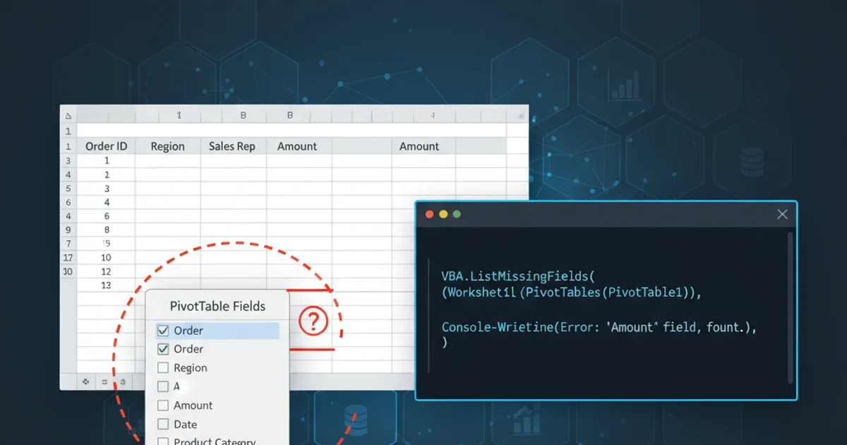
2. Identify Duplicate Headers
Duplicate headers are a common culprit. Excel needs unique names to differentiate fields. If you have two columns named 'Date', for example, Excel might only show one or behave unpredictably. Rename one of the duplicate headers (e.g., 'Order Date', 'Ship Date').
3. Convert to an Excel Table (Recommended)
While not strictly required, converting your data range into an official Excel Table (Insert > Table) is highly recommended. Excel Tables automatically manage data ranges, making it easier for Pivot Tables to detect new columns or rows. This also ensures headers are properly recognized.
Solution 2: Verify and Update the Pivot Table Data Source
Sometimes, the Pivot Table's data source might not encompass all the columns you've added or modified in your original data. This is especially true if you initially created the Pivot Table from a smaller range and then expanded your source data.
1. Access Pivot Table Options
Click anywhere inside your Pivot Table. This will activate the 'PivotTable Analyze' (or 'Options') tab on the Excel ribbon.
2. Change Data Source
In the 'PivotTable Analyze' tab, locate the 'Data' group and click 'Change Data Source'. A dialog box will appear showing the current range or table name used by your Pivot Table.
3. Select the Correct Range
Carefully select the entire range of your source data, including all headers and all rows. If you're using an Excel Table, simply type the table name (e.g., Table1) into the 'Table/Range' field. Click 'OK'.
4. Refresh the Pivot Table
After changing the data source, right-click on the Pivot Table and select 'Refresh' (or go to 'PivotTable Analyze' > 'Refresh'). This forces the Pivot Table to re-read the data and update its field list.
Solution 3: Check for Hidden Columns or Filters in Source Data
While hidden columns themselves don't usually prevent fields from appearing in the PivotTable Fields list, they can sometimes obscure issues with headers or data integrity. It's good practice to ensure your source data is fully visible when troubleshooting.
1. Unhide All Columns and Rows
Go to your source data sheet. Select the entire worksheet (click the triangle at the intersection of row and column headers, or press Ctrl+A). Right-click on any column header and select 'Unhide'. Do the same for rows.
2. Clear All Filters
Ensure no filters are applied to your source data that might be hiding relevant columns or rows. Go to 'Data' tab > 'Sort & Filter' group > 'Clear'.
3. Re-check Headers and Data Source
After unhiding and clearing filters, re-verify your column headers for uniqueness and completeness. Then, follow the steps in Solution 2 to update and refresh your Pivot Table's data source.