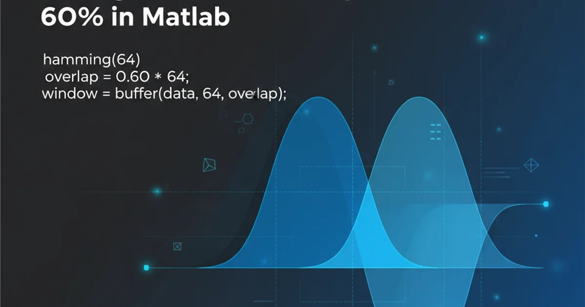
To create Hamming window of length 64 with overlap 60% in Matlab

Creating a Hamming Window with 60% Overlap in MATLAB

Learn how to generate a Hamming window of a specific length and apply a 60% overlap for signal processing applications in MATLAB.

Hamming windows are widely used in digital signal processing for spectral analysis, filter design, and other applications where reducing spectral leakage is crucial. When analyzing continuous signals in segments, applying an overlap between consecutive windows is a common practice to ensure that no data is lost at the segment boundaries and to improve the spectral estimation quality. This article will guide you through creating a Hamming window of length 64 with a 60% overlap in MATLAB.

Understanding Hamming Windows and Overlap

A Hamming window is a type of tapering window function that smoothly brings the signal to zero at its edges, thereby minimizing the abrupt transitions that can cause spectral leakage. The formula for a Hamming window of length N is given by:

w(n) = 0.54 - 0.46 * cos((2 * pi * n) / (N - 1)) for 0 <= n <= N - 1

Overlap, in the context of windowing, refers to the portion of consecutive data segments that share common samples. A 60% overlap means that 60% of the samples in the current window are also present in the previous window. This technique is particularly useful in applications like Short-Time Fourier Transform (STFT) where it helps maintain continuity and reduces artifacts caused by windowing.

flowchart TD
    A[Input Signal] --> B{Segment Signal}
    B --> C[Apply Window Function (Hamming)]
    C --> D{Calculate Overlap Samples}
    D --> E[Shift Window by (Window Length - Overlap Samples)]
    E --> F{Process Segment}
    F --> B

Workflow for windowing with overlap in signal processing

Generating a Hamming Window in MATLAB

MATLAB provides a convenient hamming function to generate Hamming windows. To create a Hamming window of length 64, you simply call hamming(64). The challenge then lies in correctly applying the 60% overlap when processing a longer signal. This involves calculating the number of non-overlapping samples (hop size) and iterating through the signal, extracting segments, applying the window, and advancing by the hop size.

% Define window parameters
windowLength = 64; % Length of the Hamming window
overlapPercentage = 0.60; % 60% overlap

% Generate the Hamming window
hammingWindow = hamming(windowLength);

% Display the first few values and plot the window
disp('First 5 values of the Hamming window:');
disp(hammingWindow(1:5));

figure;
plot(hammingWindow);
title('Hamming Window of Length 64');
xlabel('Sample Index');
ylabel('Amplitude');
grid on;

MATLAB code to generate and visualize a Hamming window of length 64.

Implementing 60% Overlap for Signal Processing

To apply the 60% overlap, we first need to calculate the number of samples that will overlap between consecutive windows. If the window length is N and the overlap percentage is P, the number of overlapping samples is N * P. The hop size, or the number of samples to advance for the next window, is then N - (N * P). For a 64-sample window with 60% overlap, the overlap samples would be 64 * 0.60 = 38.4. Since samples must be integers, we typically round this to the nearest integer, or specifically, floor for overlap samples to ensure the hop size is an integer. The hop size would then be 64 - floor(38.4) = 64 - 38 = 26 samples. This means each new window starts 26 samples after the previous one.

% Assume a dummy signal for demonstration
samplingFreq = 1000; % Hz
time = 0:1/samplingFreq:1-1/samplingFreq; % 1 second duration
signal = sin(2*pi*50*time) + 0.5*randn(size(time)); % 50 Hz sine + noise

% Window and overlap parameters
windowLength = 64;
overlapPercentage = 0.60;

% Calculate overlap samples and hop size
overlapSamples = round(windowLength * overlapPercentage); % Round to nearest integer
hopSize = windowLength - overlapSamples;

disp(['Window Length: ', num2str(windowLength)]);
disp(['Overlap Samples: ', num2str(overlapSamples)]);
disp(['Hop Size: ', num2str(hopSize)]);

% Initialize a cell array to store windowed segments
windowedSegments = {};

% Iterate through the signal with overlap
startIndex = 1;
while startIndex + windowLength - 1 <= length(signal)
    endIndex = startIndex + windowLength - 1;
    currentSegment = signal(startIndex:endIndex);
    
    % Apply the Hamming window
    windowedSegment = currentSegment .* hamming(windowLength);
    
    windowedSegments{end+1} = windowedSegment; %#ok<AGROW>
    
    % Move to the next segment
    startIndex = startIndex + hopSize;
end

disp(['Number of windowed segments: ', num2str(length(windowedSegments))]);

% Plot the first few windowed segments (optional)
if ~isempty(windowedSegments)
    figure;
    for i = 1:min(3, length(windowedSegments)) % Plot first 3 segments
        subplot(3,1,i);
        plot(windowedSegments{i});
        title(['Windowed Segment ', num2str(i)]);
        xlabel('Sample Index');
        ylabel('Amplitude');
        grid on;
    end
end

MATLAB code demonstrating the application of a Hamming window with 60% overlap to a sample signal.

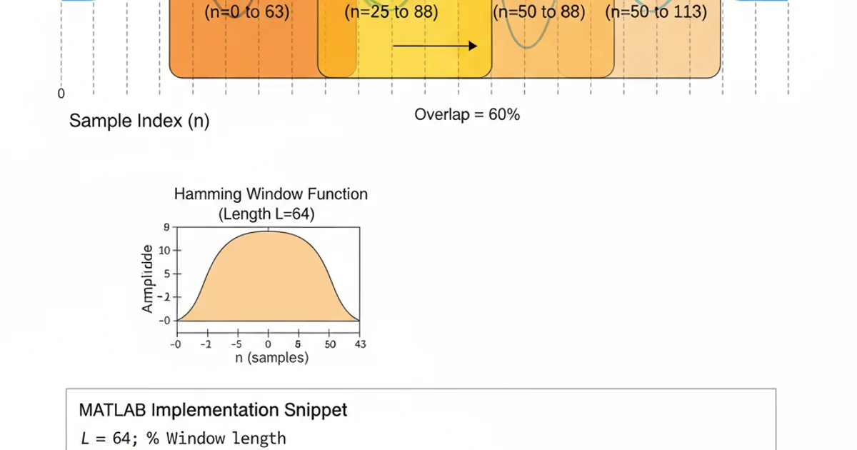
Visual representation of a signal being segmented with overlapping windows.

This approach allows for robust analysis of signals by ensuring that transient events or features occurring at segment boundaries are not missed. The choice of window length and overlap percentage often depends on the specific characteristics of the signal and the requirements of the analysis, such as frequency resolution and time localization.