Remove leading or trailing spaces in an entire column of data

Efficiently Remove Leading or Trailing Spaces from Excel Columns

Learn how to clean your Excel data by removing unwanted leading or trailing spaces from an entire column using built-in functions and practical formulas.

Unwanted leading or trailing spaces in Excel can cause numerous issues, from incorrect lookups and filters to messy data presentation. These spaces, often introduced during data entry or import, are invisible but can significantly impact data integrity and analysis. This article will guide you through effective methods to clean your Excel columns, ensuring your data is precise and ready for use.

Understanding the Problem: Invisible Spaces

Before diving into solutions, it's crucial to understand why these spaces are problematic. Excel treats ' Apple' and 'Apple ' as different values from 'Apple'. This distinction can lead to failed VLOOKUPs, inaccurate COUNTIF results, and sorting errors. Identifying these spaces visually is nearly impossible, making programmatic solutions essential.

flowchart TD
    A[Data Entry/Import] --> B{Leading/Trailing Spaces Introduced?}
    B -- Yes --> C[Data Inconsistency]
    C --> D{"VLOOKUP" Fails?}
    C --> E{"COUNTIF" Inaccurate?}
    C --> F[Sorting Errors]
    D --> G[Analysis Impacted]
    E --> G
    F --> G
    B -- No --> H[Clean Data]
    H --> I[Accurate Analysis]

Impact of Leading/Trailing Spaces on Data Integrity

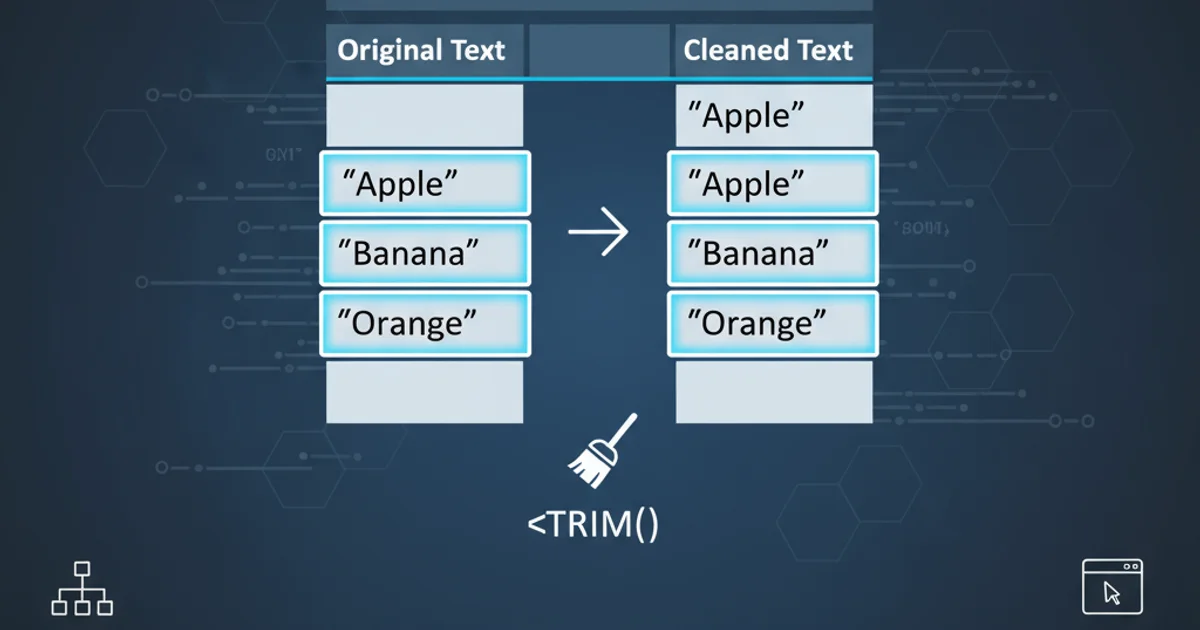
Method 1: Using the TRIM Function

The TRIM function in Excel is specifically designed to remove all spaces from text except for single spaces between words. It's the most straightforward and commonly used method for cleaning leading and trailing spaces. This function is ideal when you want to ensure there's only one space between words and no spaces at the beginning or end of a text string.

=TRIM(A1)

Applying the TRIM function to cell A1

1. Insert a New Column

To avoid overwriting your original data, insert a new, empty column adjacent to the column you wish to clean. For example, if your data is in column A, insert a new column B.

2. Apply the TRIM Formula

In the first cell of your new column (e.g., B1), enter the formula =TRIM(A1), assuming your data starts in A1. Press Enter.

3. Fill Down the Formula

Select cell B1, then drag the fill handle (the small square at the bottom-right corner of the cell) down to apply the formula to all relevant rows in column B. Alternatively, double-click the fill handle to auto-fill.

4. Copy and Paste as Values

Select the entire new column (e.g., B), copy it (Ctrl+C), then select the original column (e.g., A), right-click, and choose 'Paste Special' -> 'Values'. This replaces the original data with the cleaned values, removing the formulas.

5. Delete the Helper Column

Once the cleaned data is pasted as values into the original column, you can delete the helper column (e.g., B).

Method 2: Using FIND/REPLACE for Specific Characters (Advanced)

While TRIM is excellent for standard spaces, sometimes data might contain non-breaking spaces (ASCII character 160) or other invisible characters that TRIM doesn't handle. In such cases, a combination of CLEAN and SUBSTITUTE or the Find/Replace feature can be more effective.

=TRIM(CLEAN(SUBSTITUTE(A1,CHAR(160)," ")))

Formula to remove non-breaking spaces and then trim

This formula first replaces all non-breaking spaces (CHAR(160)) with regular spaces, then CLEAN removes non-printable characters, and finally TRIM handles leading/trailing spaces and multiple spaces between words.

Method 3: Using Power Query (Excel 2010 onwards with Add-in, Built-in for 2016+)

For larger datasets or recurring cleaning tasks, Power Query offers a more robust and automated solution. It allows you to transform data without altering the original source and can be refreshed easily.

1. Load Data into Power Query

Select your data range or table. Go to 'Data' tab -> 'Get & Transform Data' group -> 'From Table/Range' (Excel 2016+) or 'From Other Sources' -> 'From Table' (Excel 2010/2013 with Power Query Add-in).

2. Transform the Column

In the Power Query Editor, select the column you want to clean. Go to 'Transform' tab -> 'Text Column' group -> 'Format' -> 'Trim'. This will remove leading and trailing spaces.

3. Apply Additional Cleaning (Optional)

If you suspect other invisible characters, you can also use 'Format' -> 'Clean' in Power Query to remove non-printable characters.

4. Load Data Back to Excel

Once satisfied with the transformation, go to 'Home' tab -> 'Close & Load' -> 'Close & Load To...'. Choose where you want to load the cleaned data (e.g., a new worksheet or replace the existing one).